
Sorting Algorithm
A sorting algorithm is used to arrange elements of an array/list in a specific order. For example,
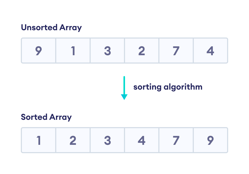
Here, we are sorting the array in ascending order.
There are various sorting algorithms that can be used to complete this operation. And, we can use any algorithm based on the requirement.
Different Sorting Algorithms
- Bubble Sort
- Selection Sort
- Insertion Sort
- Merge Sort
- Quicksort
- Counting Sort
- Radix Sort
- Bucket Sort
- Heap Sort
- Shell Sort
Complexity of Sorting Algorithms
The efficiency of any sorting algorithm is determined by the time complexity and space complexity of the algorithm.
1. Time Complexity: Time complexity refers to the time taken by an algorithm to complete its execution with respect to the size of the input. It can be represented in different forms:
2. Space Complexity: Space complexity refers to the total amount of memory used by the algorithm for a complete execution. It includes both the auxiliary memory and the input.
The auxiliary memory is the additional space occupied by the algorithm apart from the input data. Usually, auxiliary memory is considered for calculating the space complexity of an algorithm.
Let's see a complexity analysis of different sorting algorithms.
| Sorting Algorithm | Time Complexity - Best | Time Complexity - Worst | Time Complexity - Average | Space Complexity |
|---|---|---|---|---|
| Bubble Sort | n | n2 | n2 | 1 |
| Selection Sort | n2 | n2 | n2 | 1 |
| Insertion Sort | n | n2 | n2 | 1 |
| Merge Sort | nlog n | nlog n | nlog n | n |
| Quicksort | nlog n | n2 | nlog n | log n |
| Counting Sort | n+k | n+k | n+k | max |
| Radix Sort | n+k | n+k | n+k | max |
| Bucket Sort | n+k | n2 | n | n+k |
| Heap Sort | nlog n | nlog n | nlog n | 1 |
| Shell Sort | nlog n | n2 | nlog n | 1 |
Stability of Sorting Algorithm
A sorting algorithm is considered stable if the two or more items with the same value maintain the same relative positions even after sorting.
For example, in the image below, there are two items with the same value 3. An unstable sorting algorithm allows two possibilities where the two positions of 3 may or may not be maintained.
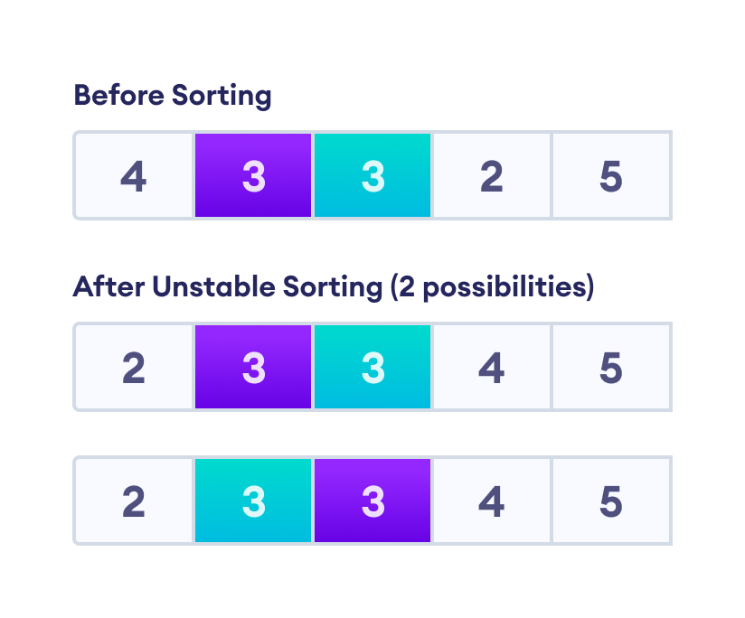
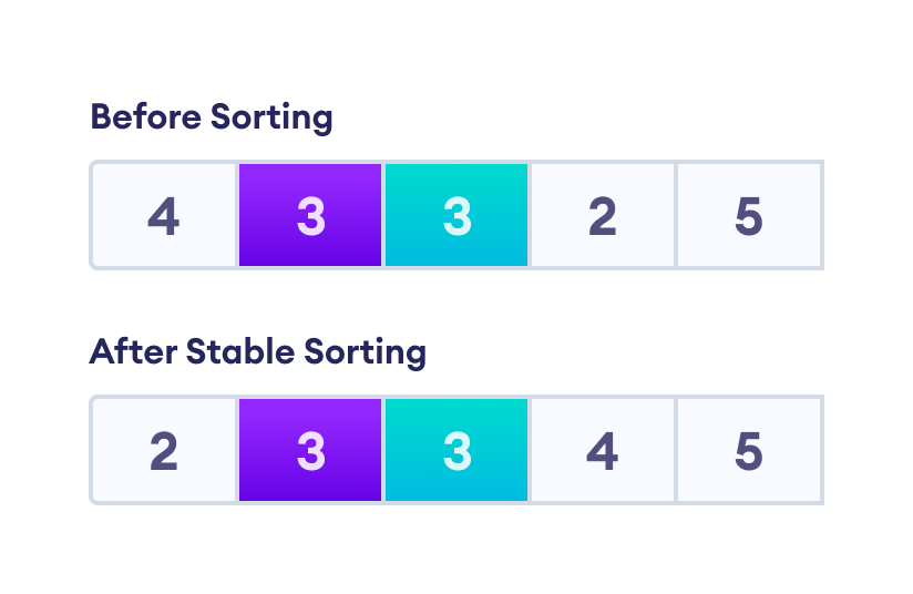
However, after a stable sorting algorithm, there is always one possibility where the positions are maintained as in the original array.
Here's a table showing the stablilty of different sorting algorithm.
| Sorting Algorithm | Stability |
|---|---|
| Bubble Sort | Yes |
| Selection Sort | No |
| Insertion Sort | Yes |
| Merge Sort | Yes |
| Quicksort | No |
| Counting Sort | Yes |
| Radix Sort | Yes |
| Bucket Sort | Yes |
| Heap Sort | No |
| Shell Sort | No |
Bucket Sort Algorithm
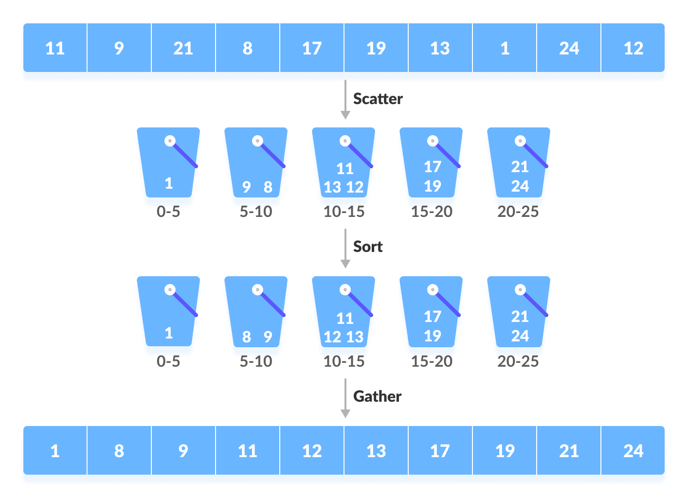
Bucket Sort is a sorting algorithm that divides the unsorted array elements into several groups called buckets. Each bucket is then sorted by using any of the suitable sorting algorithms or recursively applying the same bucket algorithm.
Finally, the sorted buckets are combined to form a final sorted array.
Scatter Gather Approach
The process of bucket sort can be understood as a scatter-gather approach. Here, elements are first scattered into buckets then the elements in each bucket are sorted. Finally, the elements are gathered in order.
Working of Bucket Sort
- Suppose, the input array is:

Input array
Create an array of size 10. Each slot of this array is used as a bucket for storing elements.
Array in which each position is a bucket - Insert elements into the buckets from the array. The elements are inserted according to the range of the bucket.
In our example code, we have buckets each of ranges from 0 to 1, 1 to 2, 2 to 3,...... (n-1) to n.
Suppose, an input element is.23is taken. It is multiplied bysize = 10(ie..23*10=2.3). Then, it is converted into an integer (ie.2.3≈2). Finally, .23 is inserted into bucket-2.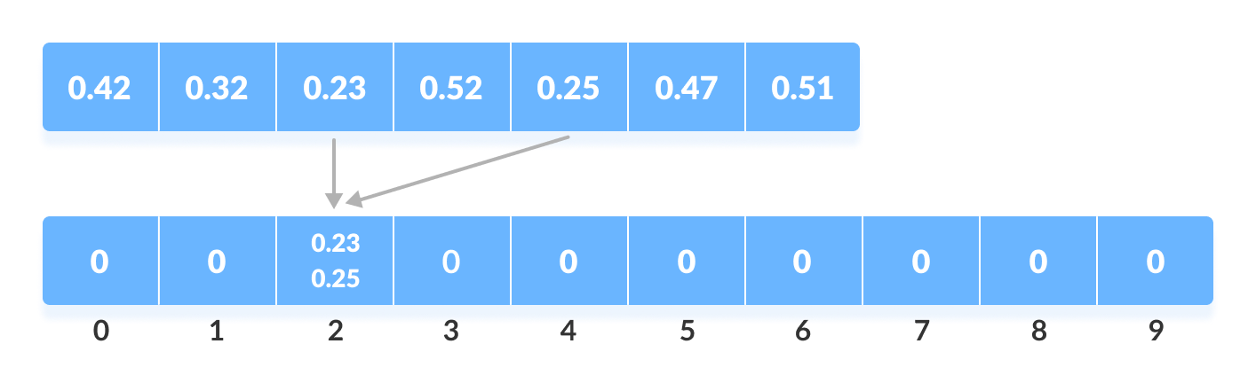
Insert elements into the buckets from the array
Similarly, .25 is also inserted into the same bucket. Everytime, the floor value of the floating point number is taken.
If we take integer numbers as input, we have to divide it by the interval (10 here) to get the floor value.
Similarly, other elements are inserted into their respective buckets.
Insert all the elements into the buckets from the array - The elements of each bucket are sorted using any of the stable sorting algorithms. Here, we have used quicksort (inbuilt function).

Sort the elements in each bucket - The elements from each bucket are gathered.
It is done by iterating through the bucket and inserting an individual element into the original array in each cycle. The element from the bucket is erased once it is copied into the original array.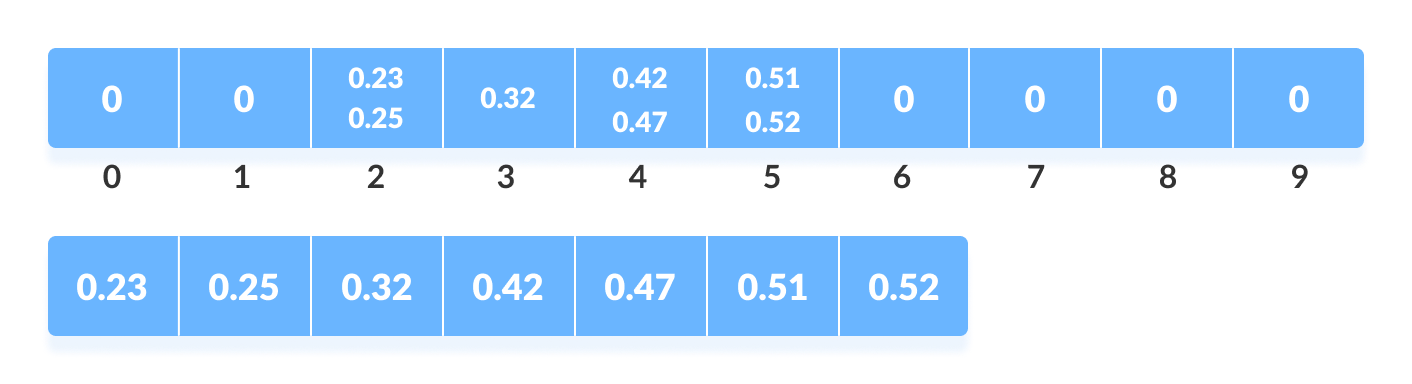
Gather elements from each bucket
Bucket Sort Algorithm
bucketSort()
  create N buckets each of which can hold a range of values
  for all the buckets
    initialize each bucket with 0 values
  for all the buckets
    put elements into buckets matching the range
  for all the buckets
    sort elements in each bucket
  gather elements from each bucket
end bucketSort
Bucket Sort Code in Python, Java, and C/C++
# Bucket Sort in Python


def bucketSort(array):
    bucket = []

    # Create empty buckets
    for i in range(len(array)):
        bucket.append([])

    # Insert elements into their respective buckets
    for j in array:
        index_b = int(10 * j)
        bucket[index_b].append(j)

    # Sort the elements of each bucket
    for i in range(len(array)):
        bucket[i] = sorted(bucket[i])

    # Get the sorted elements
    k = 0
    for i in range(len(array)):
        for j in range(len(bucket[i])):
            array[k] = bucket[i][j]
            k += 1
    return array


array = [.42, .32, .33, .52, .37, .47, .51]
print("Sorted Array in descending order is")
print(bucketSort(array))
// Bucket sort in Java

import java.util.ArrayList;
import java.util.Collections;

public class BucketSort {
  public void bucketSort(float[] arr, int n) {
    if (n <= 0)
      return;
    @SuppressWarnings("unchecked")
    ArrayList<Float>[] bucket = new ArrayList[n];

    // Create empty buckets
    for (int i = 0; i < n; i++)
      bucket[i] = new ArrayList<Float>();

    // Add elements into the buckets
    for (int i = 0; i < n; i++) {
      int bucketIndex = (int) arr[i] * n;
      bucket[bucketIndex].add(arr[i]);
    }

    // Sort the elements of each bucket
    for (int i = 0; i < n; i++) {
      Collections.sort((bucket[i]));
    }

    // Get the sorted array
    int index = 0;
    for (int i = 0; i < n; i++) {
      for (int j = 0, size = bucket[i].size(); j < size; j++) {
        arr[index++] = bucket[i].get(j);
      }
    }
  }

  // Driver code
  public static void main(String[] args) {
    BucketSort b = new BucketSort();
    float[] arr = { (float) 0.42, (float) 0.32, (float) 0.33, (float) 0.52, (float) 0.37, (float) 0.47,
        (float) 0.51 };
    b.bucketSort(arr, 7);

    for (float i : arr)
      System.out.print(i + "  ");
  }
}
// Bucket sort in C

#include <stdio.h>
#include <stdlib.h>

#define NARRAY 7   // Array size
#define NBUCKET 6  // Number of buckets
#define INTERVAL 10  // Each bucket capacity

struct Node {
  int data;
  struct Node *next;
};

void BucketSort(int arr[]);
struct Node *InsertionSort(struct Node *list);
void print(int arr[]);
void printBuckets(struct Node *list);
int getBucketIndex(int value);

// Sorting function
void BucketSort(int arr[]) {
  int i, j;
  struct Node **buckets;

  // Create buckets and allocate memory size
  buckets = (struct Node **)malloc(sizeof(struct Node *) * NBUCKET);

  // Initialize empty buckets
  for (i = 0; i < NBUCKET; ++i) {
    buckets[i] = NULL;
  }

  // Fill the buckets with respective elements
  for (i = 0; i < NARRAY; ++i) {
    struct Node *current;
    int pos = getBucketIndex(arr[i]);
    current = (struct Node *)malloc(sizeof(struct Node));
    current->data = arr[i];
    current->next = buckets[pos];
    buckets[pos] = current;
  }

  // Print the buckets along with their elements
  for (i = 0; i < NBUCKET; i++) {
    printf("Bucket[%d]: ", i);
    printBuckets(buckets[i]);
    printf("\n");
  }

  // Sort the elements of each bucket
  for (i = 0; i < NBUCKET; ++i) {
    buckets[i] = InsertionSort(buckets[i]);
  }

  printf("-------------\n");
  printf("Bucktets after sorting\n");
  for (i = 0; i < NBUCKET; i++) {
    printf("Bucket[%d]: ", i);
    printBuckets(buckets[i]);
    printf("\n");
  }

  // Put sorted elements on arr
  for (j = 0, i = 0; i < NBUCKET; ++i) {
    struct Node *node;
    node = buckets[i];
    while (node) {
      arr[j++] = node->data;
      node = node->next;
    }
  }

  return;
}

// Function to sort the elements of each bucket
struct Node *InsertionSort(struct Node *list) {
  struct Node *k, *nodeList;
  if (list == 0 || list->next == 0) {
    return list;
  }

  nodeList = list;
  k = list->next;
  nodeList->next = 0;
  while (k != 0) {
    struct Node *ptr;
    if (nodeList->data > k->data) {
      struct Node *tmp;
      tmp = k;
      k = k->next;
      tmp->next = nodeList;
      nodeList = tmp;
      continue;
    }

    for (ptr = nodeList; ptr->next != 0; ptr = ptr->next) {
      if (ptr->next->data > k->data)
        break;
    }

    if (ptr->next != 0) {
      struct Node *tmp;
      tmp = k;
      k = k->next;
      tmp->next = ptr->next;
      ptr->next = tmp;
      continue;
    } else {
      ptr->next = k;
      k = k->next;
      ptr->next->next = 0;
      continue;
    }
  }
  return nodeList;
}

int getBucketIndex(int value) {
  return value / INTERVAL;
}

void print(int ar[]) {
  int i;
  for (i = 0; i < NARRAY; ++i) {
    printf("%d ", ar[i]);
  }
  printf("\n");
}

// Print buckets
void printBuckets(struct Node *list) {
  struct Node *cur = list;
  while (cur) {
    printf("%d ", cur->data);
    cur = cur->next;
  }
}

// Driver code
int main(void) {
  int array[NARRAY] = {42, 32, 33, 52, 37, 47, 51};

  printf("Initial array: ");
  print(array);
  printf("-------------\n");

  BucketSort(array);
  printf("-------------\n");
  printf("Sorted array: ");
  print(array);
  return 0;
}
// Bucket sort in C++

#include <iomanip>
#include <iostream>
using namespace std;

#define NARRAY 7   // Array size
#define NBUCKET 6  // Number of buckets
#define INTERVAL 10  // Each bucket capacity

struct Node {
  int data;
  struct Node *next;
};

void BucketSort(int arr[]);
struct Node *InsertionSort(struct Node *list);
void print(int arr[]);
void printBuckets(struct Node *list);
int getBucketIndex(int value);

// Sorting function
void BucketSort(int arr[]) {
  int i, j;
  struct Node **buckets;

  // Create buckets and allocate memory size
  buckets = (struct Node **)malloc(sizeof(struct Node *) * NBUCKET);

  // Initialize empty buckets
  for (i = 0; i < NBUCKET; ++i) {
    buckets[i] = NULL;
  }

  // Fill the buckets with respective elements
  for (i = 0; i < NARRAY; ++i) {
    struct Node *current;
    int pos = getBucketIndex(arr[i]);
    current = (struct Node *)malloc(sizeof(struct Node));
    current->data = arr[i];
    current->next = buckets[pos];
    buckets[pos] = current;
  }

  // Print the buckets along with their elements
  for (i = 0; i < NBUCKET; i++) {
    cout << "Bucket[" << i << "] : ";
    printBuckets(buckets[i]);
    cout << endl;
  }

  // Sort the elements of each bucket
  for (i = 0; i < NBUCKET; ++i) {
    buckets[i] = InsertionSort(buckets[i]);
  }

  cout << "-------------" << endl;
  cout << "Bucktets after sorted" << endl;
  for (i = 0; i < NBUCKET; i++) {
    cout << "Bucket[" << i << "] : ";
    printBuckets(buckets[i]);
    cout << endl;
  }

  // Put sorted elements on arr
  for (j = 0, i = 0; i < NBUCKET; ++i) {
    struct Node *node;
    node = buckets[i];
    while (node) {
      arr[j++] = node->data;
      node = node->next;
    }
  }

  for (i = 0; i < NBUCKET; ++i) {
    struct Node *node;
    node = buckets[i];
    while (node) {
      struct Node *tmp;
      tmp = node;
      node = node->next;
      free(tmp);
    }
  }
  free(buckets);
  return;
}

// Function to sort the elements of each bucket
struct Node *InsertionSort(struct Node *list) {
  struct Node *k, *nodeList;
  if (list == 0 || list->next == 0) {
    return list;
  }

  nodeList = list;
  k = list->next;
  nodeList->next = 0;
  while (k != 0) {
    struct Node *ptr;
    if (nodeList->data > k->data) {
      struct Node *tmp;
      tmp = k;
      k = k->next;
      tmp->next = nodeList;
      nodeList = tmp;
      continue;
    }

    for (ptr = nodeList; ptr->next != 0; ptr = ptr->next) {
      if (ptr->next->data > k->data)
        break;
    }

    if (ptr->next != 0) {
      struct Node *tmp;
      tmp = k;
      k = k->next;
      tmp->next = ptr->next;
      ptr->next = tmp;
      continue;
    } else {
      ptr->next = k;
      k = k->next;
      ptr->next->next = 0;
      continue;
    }
  }
  return nodeList;
}

int getBucketIndex(int value) {
  return value / INTERVAL;
}

// Print buckets
void print(int ar[]) {
  int i;
  for (i = 0; i < NARRAY; ++i) {
    cout << setw(3) << ar[i];
  }
  cout << endl;
}

void printBuckets(struct Node *list) {
  struct Node *cur = list;
  while (cur) {
    cout << setw(3) << cur->data;
    cur = cur->next;
  }
}

// Driver code
int main(void) {
  int array[NARRAY] = {42, 32, 33, 52, 37, 47, 51};

  cout << "Initial array: " << endl;
  print(array);
  cout << "-------------" << endl;

  BucketSort(array);
  cout << "-------------" << endl;
  cout << "Sorted array: " << endl;
  print(array);
}
Bucket Sort Complexity
| Time Complexity | |
|---|---|
| Best | O(n+k) |
| Worst | O(n2) |
| Average | O(n) |
| Space Complexity | O(n+k) |
| Stability | Yes |
- Worst Case Complexity:
O(n2)
When there are elements of close range in the array, they are likely to be placed in the same bucket. This may result in some buckets having more number of elements than others.
It makes the complexity depend on the sorting algorithm used to sort the elements of the bucket.
The complexity becomes even worse when the elements are in reverse order. If insertion sort is used to sort elements of the bucket, then the time complexity becomesO(n2). - Best Case Complexity:
O(n+k)
It occurs when the elements are uniformly distributed in the buckets with a nearly equal number of elements in each bucket.
The complexity becomes even better if the elements inside the buckets are already sorted.
If insertion sort is used to sort elements of a bucket then the overall complexity in the best case will be linear ie.O(n+k).O(n)is the complexity for making the buckets andO(k)is the complexity for sorting the elements of the bucket using algorithms having linear time complexity at the best case. - Average Case Complexity:
O(n)
It occurs when the elements are distributed randomly in the array. Even if the elements are not distributed uniformly, bucket sort runs in linear time. It holds true until the sum of the squares of the bucket sizes is linear in the total number of elements.
Bucket Sort Applications
Bucket sort is used when:
- input is uniformly distributed over a range.
- there are floating point values
Similar Sorting Algorithms
Shell Sort Algorithm
Shell sort is a generalized version of the insertion sort algorithm. It first sorts elements that are far apart from each other and successively reduces the interval between the elements to be sorted.
The interval between the elements is reduced based on the sequence used. Some of the optimal sequences that can be used in the shell sort algorithm are:
- Shell's original sequence:
N/2 , N/4 , …, 1 - Knuth's increments:
1, 4, 13, …, (3k– 1) / 2 - Sedgewick's increments:
1, 8, 23, 77, 281, 1073, 4193, 16577...4j+1+ 3·2j+ 1 - Hibbard's increments:
1, 3, 7, 15, 31, 63, 127, 255, 511… - Papernov & Stasevich increment:
1, 3, 5, 9, 17, 33, 65,... - Pratt:
1, 2, 3, 4, 6, 9, 8, 12, 18, 27, 16, 24, 36, 54, 81....
Note: The performance of the shell sort depends on the type of sequence used for a given input array.
Working of Shell Sort
- Suppose, we need to sort the following array.

Initial array - We are using the shell's original sequence
(N/2, N/4, ...1) as intervals in our algorithm.
In the first loop, if the array size isN = 8then, the elements lying at the interval ofN/2 = 4are compared and swapped if they are not in order.- The 0th element is compared with the 4th element.
- If the 0th element is greater than the 4th one then, the 4th element is first stored in
tempvariable and the0thelement (ie. greater element) is stored in the4thposition and the element stored intempis stored in the0thposition.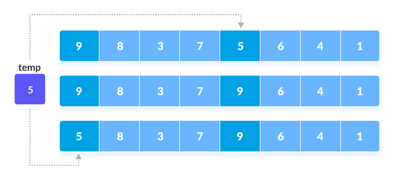
Rearrange the elements at n/2 interval
This process goes on for all the remaining elements.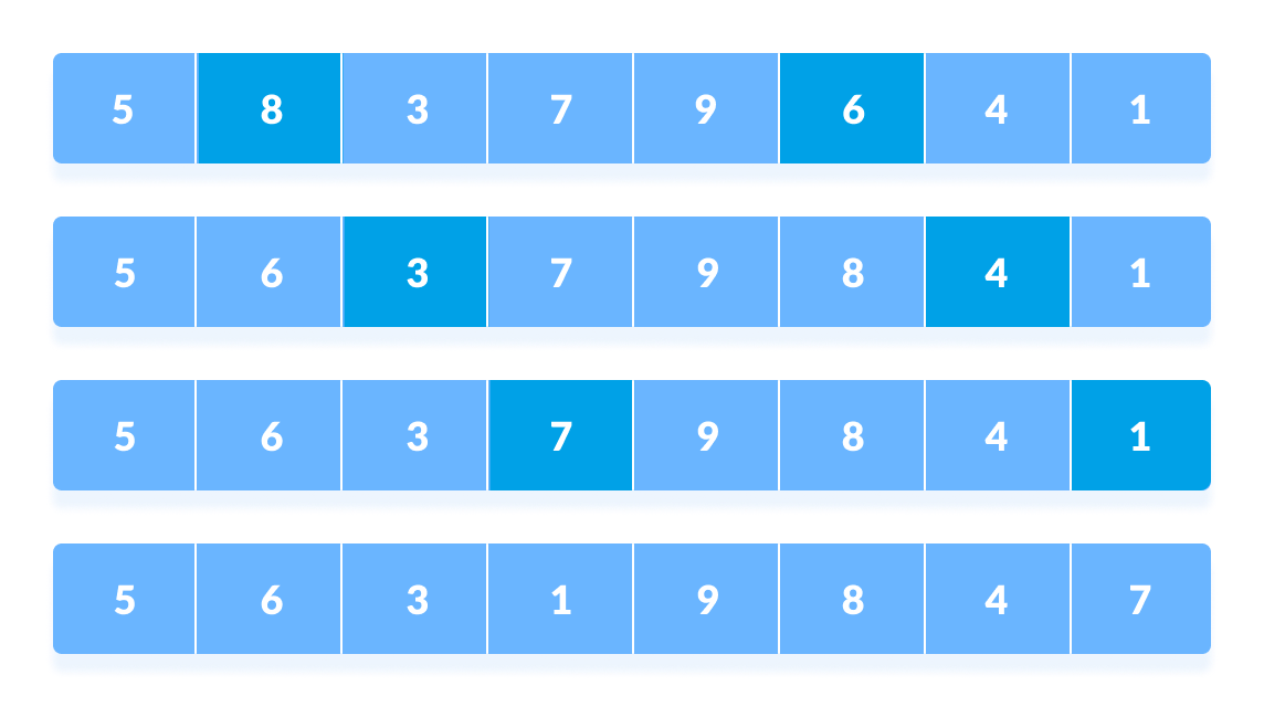
Rearrange all the elements at n/2 interval
- In the second loop, an interval of
N/4 = 8/4 = 2is taken and again the elements lying at these intervals are sorted.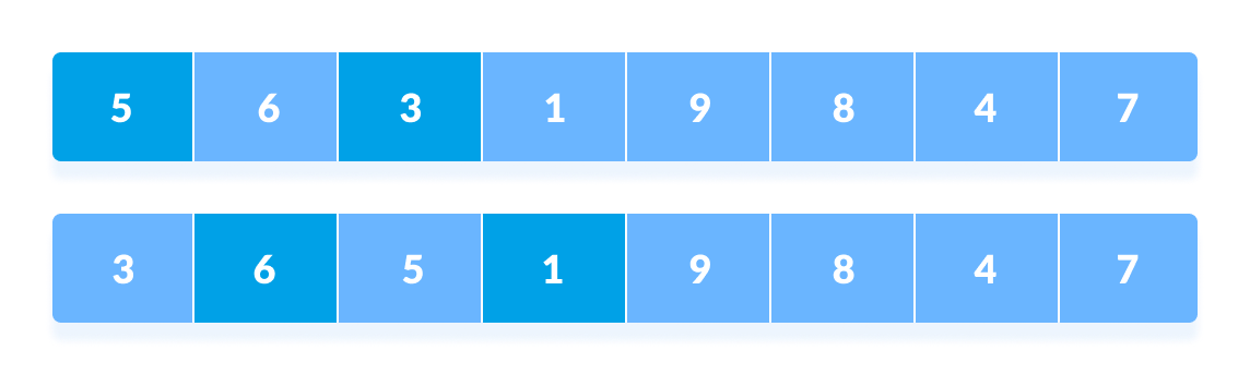
Rearrange the elements at n/4 interval
You might get confused at this point.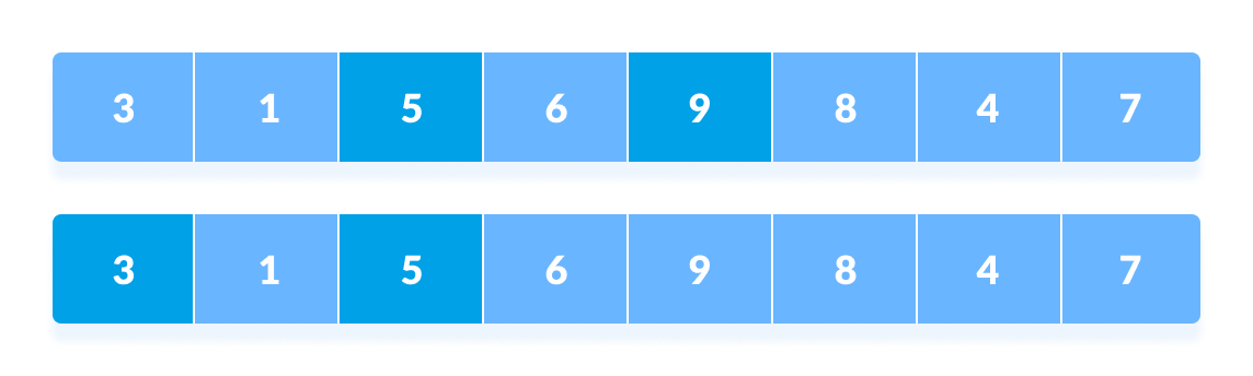
All the elements in the array lying at the current interval are compared.
The elements at 4th and2ndposition are compared. The elements at 2nd and0thposition are also compared. All the elements in the array lying at the current interval are compared. - The same process goes on for remaining elements.
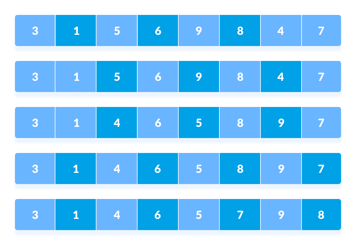
Rearrange all the elements at n/4 interval - Finally, when the interval is
N/8 = 8/8 =1then the array elements lying at the interval of 1 are sorted. The array is now completely sorted.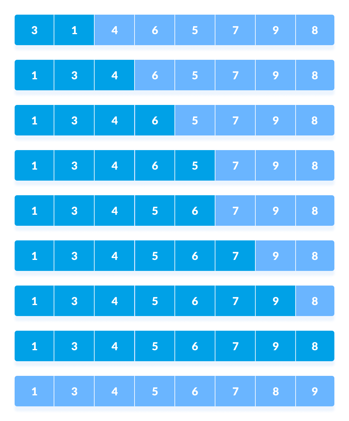
Rearrange the elements at n/8 interval
Shell Sort Algorithm
shellSort(array, size)
  for interval i <- size/2n down to 1
    for each interval "i" in array
        sort all the elements at interval "i"
end shellSort
Shell Sort Code in Python, Java, and C/C++
# Shell sort in python


def shellSort(array, n):

    # Rearrange elements at each n/2, n/4, n/8, ... intervals
    interval = n // 2
    while interval > 0:
        for i in range(interval, n):
            temp = array[i]
            j = i
            while j >= interval and array[j - interval] > temp:
                array[j] = array[j - interval]
                j -= interval

            array[j] = temp
        interval //= 2


data = [9, 8, 3, 7, 5, 6, 4, 1]
size = len(data)
shellSort(data, size)
print('Sorted Array in Ascending Order:')
print(data)
// Shell sort in Java programming

import java.util.Arrays;

// Shell sort
class ShellSort {

  // Rearrange elements at each n/2, n/4, n/8, ... intervals
  void shellSort(int array[], int n) {
  for (int interval = n / 2; interval > 0; interval /= 2) {
    for (int i = interval; i < n; i += 1) {
    int temp = array[i];
    int j;
    for (j = i; j >= interval && array[j - interval] > temp; j -= interval) {
      array[j] = array[j - interval];
    }
    array[j] = temp;
    }
  }
  }

  // Driver code
  public static void main(String args[]) {
  int[] data = { 9, 8, 3, 7, 5, 6, 4, 1 };
  int size = data.length;
  ShellSort ss = new ShellSort();
  ss.shellSort(data, size);
  System.out.println("Sorted Array in Ascending Order: ");
  System.out.println(Arrays.toString(data));
  }
}
// Shell Sort in C programming

#include <stdio.h>

// Shell sort
void shellSort(int array[], int n) {
  // Rearrange elements at each n/2, n/4, n/8, ... intervals
  for (int interval = n / 2; interval > 0; interval /= 2) {
    for (int i = interval; i < n; i += 1) {
      int temp = array[i];
      int j;
      for (j = i; j >= interval && array[j - interval] > temp; j -= interval) {
        array[j] = array[j - interval];
      }
      array[j] = temp;
    }
  }
}

// Print an array
void printArray(int array[], int size) {
  for (int i = 0; i < size; ++i) {
    printf("%d  ", array[i]);
  }
  printf("\n");
}

// Driver code
int main() {
  int data[] = {9, 8, 3, 7, 5, 6, 4, 1};
  int size = sizeof(data) / sizeof(data[0]);
  shellSort(data, size);
  printf("Sorted array: \n");
  printArray(data, size);
}
// Shell Sort in C++ programming

#include <iostream>
using namespace std;

// Shell sort
void shellSort(int array[], int n) {
  // Rearrange elements at each n/2, n/4, n/8, ... intervals
  for (int interval = n / 2; interval > 0; interval /= 2) {
    for (int i = interval; i < n; i += 1) {
      int temp = array[i];
      int j;
      for (j = i; j >= interval && array[j - interval] > temp; j -= interval) {
        array[j] = array[j - interval];
      }
      array[j] = temp;
    }
  }
}

// Print an array
void printArray(int array[], int size) {
  int i;
  for (i = 0; i < size; i++)
    cout << array[i] << " ";
  cout << endl;
}

// Driver code
int main() {
  int data[] = {9, 8, 3, 7, 5, 6, 4, 1};
  int size = sizeof(data) / sizeof(data[0]);
  shellSort(data, size);
  cout << "Sorted array: \n";
  printArray(data, size);
}
Shell Sort Complexity
| Time Complexity | |
|---|---|
| Best | O(nlog n) |
| Worst | O(n2) |
| Average | O(nlog n) |
| Space Complexity | O(1) |
| Stability | No |
Shell sort is an unstable sorting algorithm because this algorithm does not examine the elements lying in between the intervals.
Time Complexity
- Worst Case Complexity: less than or equal to
O(n2)
Worst case complexity for shell sort is always less than or equal toO(n2).
According to Poonen Theorem, worst case complexity for shell sort isΘ(Nlog N)2/(log log N)2)orΘ(Nlog N)2/log log N)orΘ(N(log N)2)or something in between. - Best Case Complexity:
O(n*log n)
When the array is already sorted, the total number of comparisons for each interval (or increment) is equal to the size of the array. - Average Case Complexity:
O(n*log n)
It is aroundO(n1.25).
The complexity depends on the interval chosen. The above complexities differ for different increment sequences chosen. Best increment sequence is unknown.
Space Complexity:
The space complexity for shell sort is O(1).
Shell Sort Applications
Shell sort is used when:
- calling a stack is overhead.
uClibclibrary uses this sort. - recursion exceeds a limit.
bzip2compressor uses it. - Insertion sort does not perform well when the close elements are far apart. Shell sort helps in reducing the distance between the close elements. Thus, there will be less number of swappings to be performed.
Other Sorting Algorithms
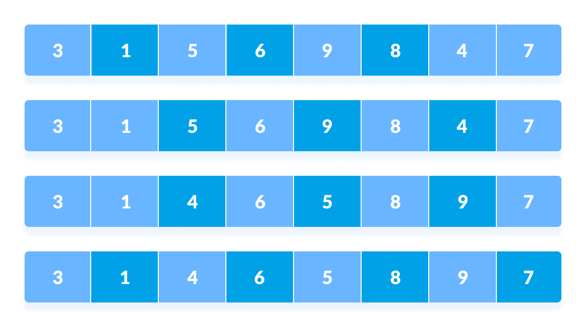
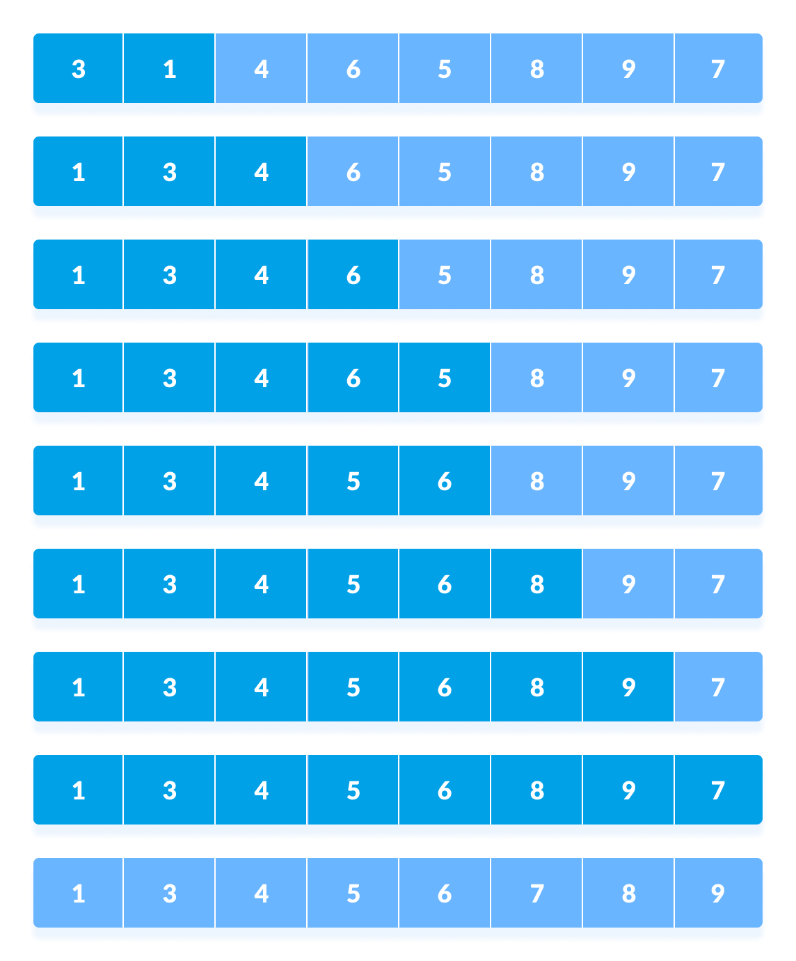
Radix Sort Algorithm
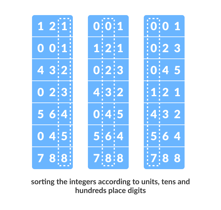
Radix sort is a sorting algorithm that sorts the elements by first grouping the individual digits of the same place value. Then, sort the elements according to their increasing/decreasing order.
Suppose, we have an array of 8 elements. First, we will sort elements based on the value of the unit place. Then, we will sort elements based on the value of the tenth place. This process goes on until the last significant place.
Let the initial array be [121, 432, 564, 23, 1, 45, 788]. It is sorted according to radix sort as shown in the figure below.
Please go through the counting sort before reading this article because counting sort is used as an intermediate sort in radix sort.
Working of Radix Sort
- Find the largest element in the array, i.e. max. Let
Xbe the number of digits inmax.Xis calculated because we have to go through all the significant places of all elements.
In this array[121, 432, 564, 23, 1, 45, 788], we have the largest number 788. It has 3 digits. Therefore, the loop should go up to hundreds place (3 times). - Now, go through each significant place one by one.
Use any stable sorting technique to sort the digits at each significant place. We have used counting sort for this.
Sort the elements based on the unit place digits (X=0).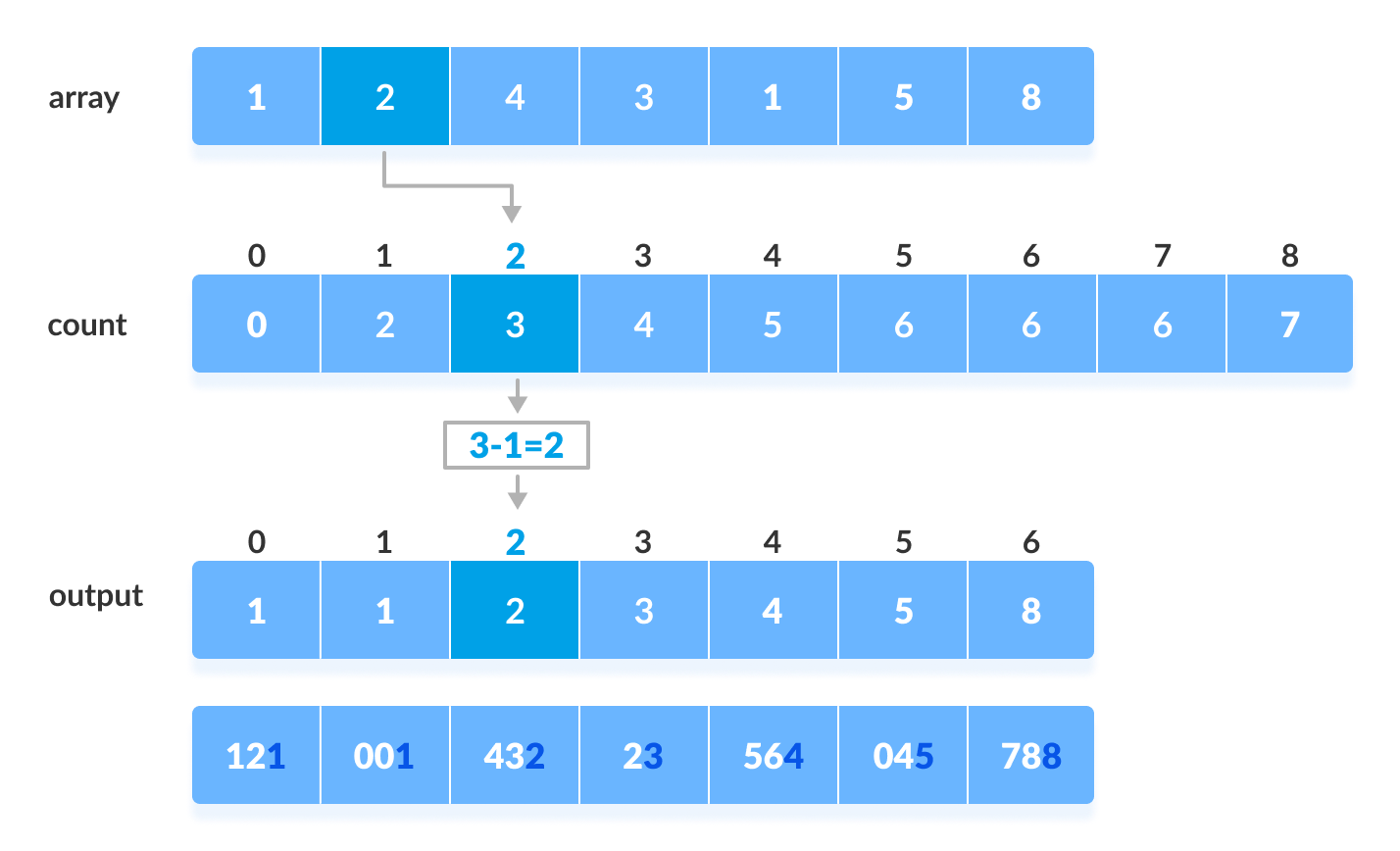
Using counting sort to sort elements based on unit place - Now, sort the elements based on digits at tens place.

Sort elements based on tens place - Finally, sort the elements based on the digits at hundreds place.

Sort elements based on hundreds place
Radix Sort Algorithm
radixSort(array)
  d <- maximum number of digits in the largest element
  create d buckets of size 0-9
  for i <- 0 to d
    sort the elements according to ith place digits using countingSort

countingSort(array, d)
  max <- find largest element among dth place elements
  initialize count array with all zeros
  for j <- 0 to size
    find the total count of each unique digit in dth place of elements and
    store the count at jth index in count array
  for i <- 1 to max
    find the cumulative sum and store it in count array itself
  for j <- size down to 1
    restore the elements to array
    decrease count of each element restored by 1
Radix Sort Code in Python, Java, and C/C++
# Radix sort in Python
# Using counting sort to sort the elements in the basis of significant places
def countingSort(array, place):
    size = len(array)
    output = [0] * size
    count = [0] * 10

    # Calculate count of elements
    for i in range(0, size):
        index = array[i] // place
        count[index % 10] += 1

    # Calculate cumulative count
    for i in range(1, 10):
        count[i] += count[i - 1]

    # Place the elements in sorted order
    i = size - 1
    while i >= 0:
        index = array[i] // place
        output[count[index % 10] - 1] = array[i]
        count[index % 10] -= 1
        i -= 1

    for i in range(0, size):
        array[i] = output[i]


# Main function to implement radix sort
def radixSort(array):
    # Get maximum element
    max_element = max(array)

    # Apply counting sort to sort elements based on place value.
    place = 1
    while max_element // place > 0:
        countingSort(array, place)
        place *= 10


data = [121, 432, 564, 23, 1, 45, 788]
radixSort(data)
print(data)
// Radix Sort in Java Programming
public class RadixSort {
    // Using counting sort to sort the elements based on significant places
    public static void countingSort(int[] array, int place) {
        int size = array.length;
        int[] output = new int[size];
        int[] count = new int[10];

        // Calculate count of elements
        for (int i = 0; i < size; i++) {
            int index = (array[i] / place) % 10;
            count[index]++;
        }
        // Calculate cumulative count
        for (int i = 1; i < 10; i++) {
            count[i] += count[i - 1];
        }
        // Place the elements in sorted order
        for (int i = size - 1; i >= 0; i--) {
            int index = (array[i] / place) % 10;
            output[count[index] - 1] = array[i];
            count[index]--;
        }
        // Copy the sorted elements into original array
        for (int i = 0; i < size; i++) {
            array[i] = output[i];
        }
    }
    // Main function to implement radix sort
    public static void radixSort(int[] array) {
        // Get maximum element
        int maxElement = getMax(array);
        // Apply counting sort to sort elements based on place value
        for (int place = 1; maxElement / place > 0; place *= 10) {
            countingSort(array, place);
        }
    }
    // A utility function to get the maximum value in the array
    public static int getMax(int[] array) {
        int max = array[0];
        for (int i = 1; i < array.length; i++) {
            if (array[i] > max) {
                max = array[i];
            }
        }
        return max;
    }
    public static void main(String[] args) {
        int[] data = {121, 432, 564, 23, 1, 45, 788};
        radixSort(data);
        System.out.println("Sorted Array in Ascending Order: ");
        for (int num : data) {
            System.out.print(num + " ");
        }
    }
}
// Radix Sort in C Programming
#include <stdio.h>
// Function to get the maximum value in the array
int getMax(int array[], int n) {
    int max = array[0];
    for (int i = 1; i < n; i++) {
        if (array[i] > max) {
            max = array[i];
        }
    }
    return max;
}
// Using counting sort to sort the elements based on significant places
void countingSort(int array[], int n, int place) {
    int output[n];
    int count[10] = {0};
    // Calculate count of elements
    for (int i = 0; i < n; i++) {
        int index = (array[i] / place) % 10;
        count[index]++;
    }
    // Calculate cumulative count
    for (int i = 1; i < 10; i++) {
        count[i] += count[i - 1];
    }
    // Place the elements in sorted order
    for (int i = n - 1; i >= 0; i--) {
        int index = (array[i] / place) % 10;
        output[count[index] - 1] = array[i];
        count[index]--;
    }
    // Copy the sorted elements into original array
    for (int i = 0; i < n; i++) {
        array[i] = output[i];
    }
}
// Main function to implement radix sort
void radixSort(int array[], int n) {
    // Get maximum element
    int maxElement = getMax(array, n);
    // Apply counting sort to sort elements based on place value
    for (int place = 1; maxElement / place > 0; place *= 10) {
        countingSort(array, n, place);
    }
}
int main() {
    int data[] = {121, 432, 564, 23, 1, 45, 788};
    int n = sizeof(data) / sizeof(data[0]);
    radixSort(data, n);
    printf("Sorted array in ascending order:\n");
    for (int i = 0; i < n; i++) {
        printf("%d ", data[i]);
    }
    return 0;
}
// Radix Sort in C++ Programming

#include <iostream>
using namespace std;

// Function to get the largest element from an array
int getMax(int array[], int n) {
  int max = array[0];
  for (int i = 1; i < n; i++)
    if (array[i] > max)
      max = array[i];
  return max;
}

// Using counting sort to sort the elements in the basis of significant places
void countingSort(int array[], int size, int place) {
  const int max = 10;
  int output[size];
  int count[max];

  for (int i = 0; i < max; ++i)
    count[i] = 0;

  // Calculate count of elements
  for (int i = 0; i < size; i++)
    count[(array[i] / place) % 10]++;

  // Calculate cumulative count
  for (int i = 1; i < max; i++)
    count[i] += count[i - 1];

  // Place the elements in sorted order
  for (int i = size - 1; i >= 0; i--) {
    output[count[(array[i] / place) % 10] - 1] = array[i];
    count[(array[i] / place) % 10]--;
  }

  for (int i = 0; i < size; i++)
    array[i] = output[i];
}

// Main function to implement radix sort
void radixsort(int array[], int size) {
  // Get maximum element
  int max = getMax(array, size);

  // Apply counting sort to sort elements based on place value.
  for (int place = 1; max / place > 0; place *= 10)
    countingSort(array, size, place);
}

// Print an array
void printArray(int array[], int size) {
  int i;
  for (i = 0; i < size; i++)
    cout << array[i] << " ";
  cout << endl;
}

// Driver code
int main() {
  int array[] = {121, 432, 564, 23, 1, 45, 788};
  int n = sizeof(array) / sizeof(array[0]);
  radixsort(array, n);
  printArray(array, n);
}
Radix Sort Complexity
| Time Complexity | |
|---|---|
| Best | O(n+k) |
| Worst | O(n+k) |
| Average | O(n+k) |
| Space Complexity | O(max) |
| Stability | Yes |
Since radix sort is a non-comparative algorithm, it has advantages over comparative sorting algorithms.
For the radix sort that uses counting sort as an intermediate stable sort, the time complexity is O(d(n+k)).
Here, d is the number cycle and O(n+k) is the time complexity of counting sort.
Thus, radix sort has linear time complexity which is better than O(nlog n) of comparative sorting algorithms.
If we take very large digit numbers or the number of other bases like 32-bit and 64-bit numbers then it can perform in linear time however the intermediate sort takes large space.
This makes radix sort space inefficient. This is the reason why this sort is not used in software libraries.
Radix Sort Applications
Radix sort is implemented in
- DC3 algorithm (Kärkkäinen-Sanders-Burkhardt) while making a suffix array.
- places where there are numbers in large ranges.
Similar Sorting Algorithms
Counting Sort Algorithm
Counting sort is a sorting algorithm that sorts the elements of an array by counting the number of occurrences of each unique element in the array. The count is stored in an auxiliary array and the sorting is done by mapping the count as an index of the auxiliary array.
Working of Counting Sort
- Find out the maximum element (let it be
max) from the given array.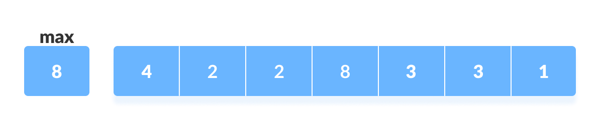
Given array - Initialize an array of length
max+1with all elements 0. This array is used for storing the count of the elements in the array.
Count array - Store the count of each element at their respective index in
countarray.
For example: if the count of element 3 is 2 then, 2 is stored in the 3rd position of count array. If element "5" is not present in the array, then 0 is stored in 5th position.
Count of each element stored - Store cumulative sum of the elements of the count array. It helps in placing the elements into the correct index of the sorted array.

Cumulative count - Find the index of each element of the original array in the count array. This gives the cumulative count. Place the element at the index calculated as shown in figure below.
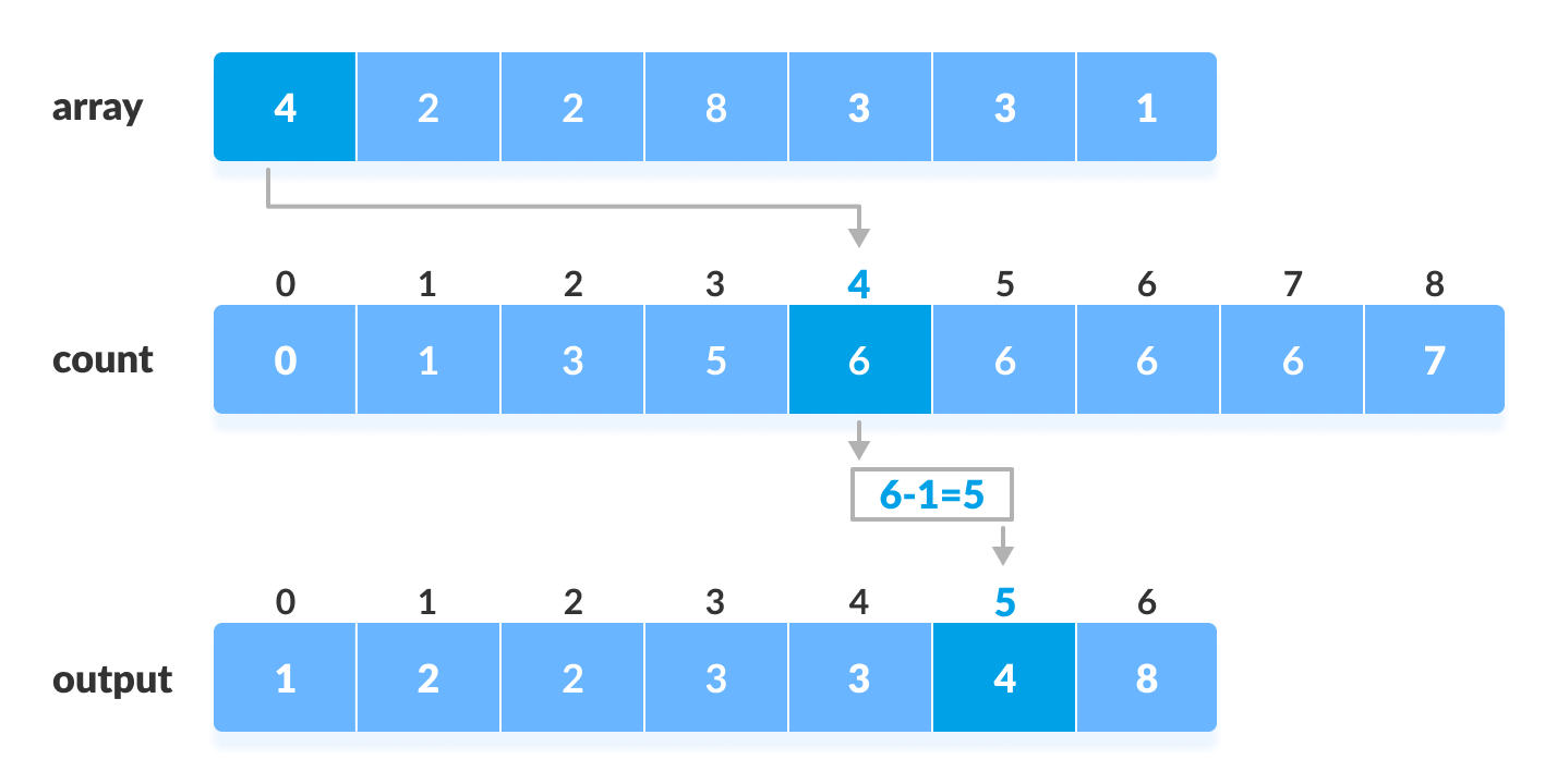
Counting sort - After placing each element at its correct position, decrease its count by one.
Counting Sort Algorithm
countingSort(array, size)
  max <- find largest element in array
  initialize count array with all zeros
  for j <- 0 to size
    find the total count of each unique element and
    store the count at jth index in count array
  for i <- 1 to max
    find the cumulative sum and store it in count array itself
  for j <- size down to 1
    restore the elements to array
    decrease count of each element restored by 1
Counting Sort Code in Python, Java, and C/C++
# Counting sort in Python programming


def countingSort(array):
    size = len(array)
    output = [0] * size

    # Initialize count array
    count = [0] * (max(array) + 1)

    # Store the count of each elements in count array
    for i in range(0, size):
        count[array[i]] += 1

    # Store the cummulative count
    for i in range(1, (max(array) + 1)):
        count[i] += count[i - 1]

    # Find the index of each element of the original array in count array
    # place the elements in output array
    i = size - 1
    while i >= 0:
        output[count[array[i]] - 1] = array[i]
        count[array[i]] -= 1
        i -= 1

    # Copy the sorted elements into original array
    for i in range(0, size):
        array[i] = output[i]


data = [4, 2, 2, 8, 3, 3, 1]
countingSort(data)
print("Sorted Array in Ascending Order: ")
print(data)
// Counting sort in Java programming

import java.util.Arrays;

class CountingSort {
  void countSort(int array[], int size) {
    int[] output = new int[size + 1];

    // Find the largest element of the array
    int max = array[0];
    for (int i = 1; i < size; i++) {
      if (array[i] > max)
        max = array[i];
    }
    int[] count = new int[max + 1];

    // Initialize count array with all zeros.
    for (int i = 0; i < max; ++i) {
      count[i] = 0;
    }

    // Store the count of each element
    for (int i = 0; i < size; i++) {
      count[array[i]]++;
    }

    // Store the cummulative count of each array
    for (int i = 1; i <= max; i++) {
      count[i] += count[i - 1];
    }

    // Find the index of each element of the original array in count array, and
    // place the elements in output array
    for (int i = size - 1; i >= 0; i--) {
      output[count[array[i]] - 1] = array[i];
      count[array[i]]--;
    }

    // Copy the sorted elements into original array
    for (int i = 0; i < size; i++) {
      array[i] = output[i];
    }
  }

  // Driver code
  public static void main(String args[]) {
    int[] data = { 4, 2, 2, 8, 3, 3, 1 };
    int size = data.length;
    CountingSort cs = new CountingSort();
    cs.countSort(data, size);
    System.out.println("Sorted Array in Ascending Order: ");
    System.out.println(Arrays.toString(data));
  }
}
// Counting sort in C programming

#include <stdio.h>

void countingSort(int array[], int size) {
  int output[10];

  // Find the largest element of the array
  int max = array[0];
  for (int i = 1; i < size; i++) {
    if (array[i] > max)
      max = array[i];
  }

  // The size of count must be at least (max+1) but
  // we cannot declare it as int count(max+1) in C as
  // it does not support dynamic memory allocation.
  // So, its size is provided statically.
  int count[10];

  // Initialize count array with all zeros.
  for (int i = 0; i <= max; ++i) {
    count[i] = 0;
  }

  // Store the count of each element
  for (int i = 0; i < size; i++) {
    count[array[i]]++;
  }

  // Store the cummulative count of each array
  for (int i = 1; i <= max; i++) {
    count[i] += count[i - 1];
  }

  // Find the index of each element of the original array in count array, and
  // place the elements in output array
  for (int i = size - 1; i >= 0; i--) {
    output[count[array[i]] - 1] = array[i];
    count[array[i]]--;
  }

  // Copy the sorted elements into original array
  for (int i = 0; i < size; i++) {
    array[i] = output[i];
  }
}

// Function to print an array
void printArray(int array[], int size) {
  for (int i = 0; i < size; ++i) {
    printf("%d  ", array[i]);
  }
  printf("\n");
}

// Driver code
int main() {
  int array[] = {4, 2, 2, 8, 3, 3, 1};
  int n = sizeof(array) / sizeof(array[0]);
  countingSort(array, n);
  printArray(array, n);
}
// Counting sort in C++ programming

#include <iostream>
using namespace std;

void countSort(int array[], int size) {
  // The size of count must be at least the (max+1) but
  // we cannot assign declare it as int count(max+1) in C++ as
  // it does not support dynamic memory allocation.
  // So, its size is provided statically.
  int output[10];
  int count[10];
  int max = array[0];

  // Find the largest element of the array
  for (int i = 1; i < size; i++) {
    if (array[i] > max)
      max = array[i];
  }

  // Initialize count array with all zeros.
  for (int i = 0; i <= max; ++i) {
    count[i] = 0;
  }

  // Store the count of each element
  for (int i = 0; i < size; i++) {
    count[array[i]]++;
  }

  // Store the cummulative count of each array
  for (int i = 1; i <= max; i++) {
    count[i] += count[i - 1];
  }

  // Find the index of each element of the original array in count array, and
  // place the elements in output array
  for (int i = size - 1; i >= 0; i--) {
    output[count[array[i]] - 1] = array[i];
    count[array[i]]--;
  }

  // Copy the sorted elements into original array
  for (int i = 0; i < size; i++) {
    array[i] = output[i];
  }
}

// Function to print an array
void printArray(int array[], int size) {
  for (int i = 0; i < size; i++)
    cout << array[i] << " ";
  cout << endl;
}

// Driver code
int main() {
  int array[] = {4, 2, 2, 8, 3, 3, 1};
  int n = sizeof(array) / sizeof(array[0]);
  countSort(array, n);
  printArray(array, n);
}
Complexity
| Time Complexity | |
|---|---|
| Best | O(n+max) |
| Worst | O(n+max) |
| Average | O(n+max) |
| Space Complexity | O(max) |
| Stability | Yes |
Time Complexities
There are mainly four main loops. (Finding the greatest value can be done outside the function.)
| for-loop | time of counting |
|---|---|
| 1st | O(max) |
| 2nd | O(size) |
| 3rd | O(max) |
| 4th | O(size) |
Overall complexity = O(max)+O(size)+O(max)+O(size) = O(max+size)
- Worst Case Complexity:
O(n+max) - Best Case Complexity:
O(n+max) - Average Case Complexity:
O(n+max)
In all the above cases, the complexity is the same because no matter how the elements are placed in the array, the algorithm goes through n+max times.
There is no comparison between any elements, so it is better than comparison based sorting techniques. But, it is bad if the integers are very large because the array of that size should be made.
Space Complexity
The space complexity of Counting Sort is O(max). Larger the range of elements, larger is the space complexity.
Counting Sort Applications
Counting sort is used when:
- there are smaller integers with multiple counts.
- linear complexity is the need.
Similar Sorting Algorithms
Quicksort Algorithm
Quicksort is a sorting algorithm based on the divide and conquer approach where
- An array is divided into subarrays by selecting a pivot element (element selected from the array).
While dividing the array, the pivot element should be positioned in such a way that elements less than pivot are kept on the left side and elements greater than pivot are on the right side of the pivot. - The left and right subarrays are also divided using the same approach. This process continues until each subarray contains a single element.
- At this point, elements are already sorted. Finally, elements are combined to form a sorted array.
Working of Quicksort Algorithm
1. Select the Pivot Element
There are different variations of quicksort where the pivot element is selected from different positions. Here, we will be selecting the rightmost element of the array as the pivot element.

2. Rearrange the Array
Now the elements of the array are rearranged so that elements that are smaller than the pivot are put on the left and the elements greater than the pivot are put on the right.

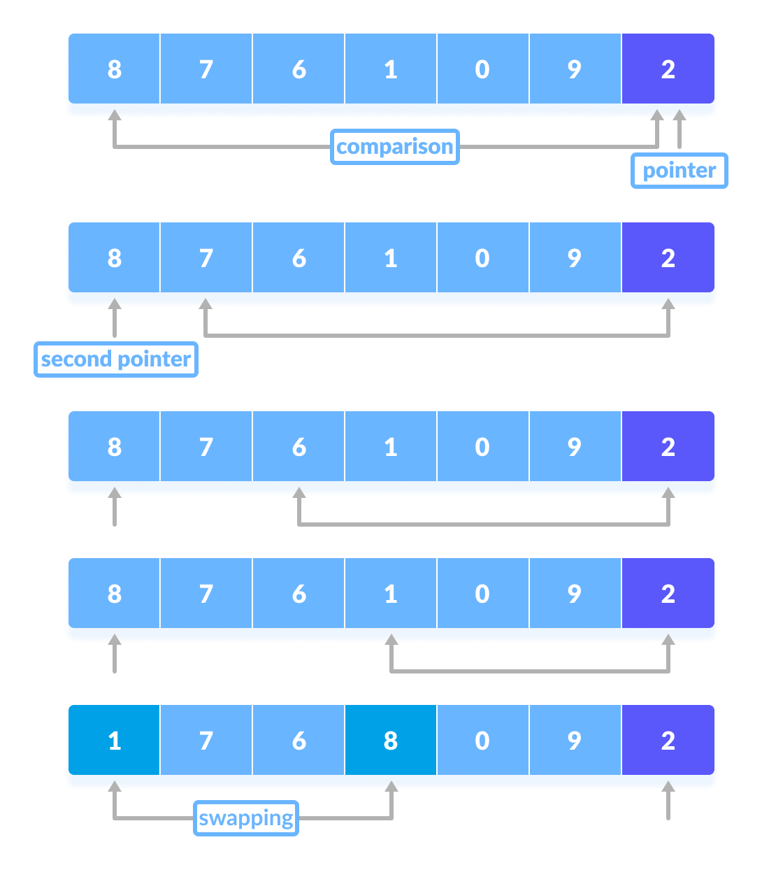
Here's how we rearrange the array:
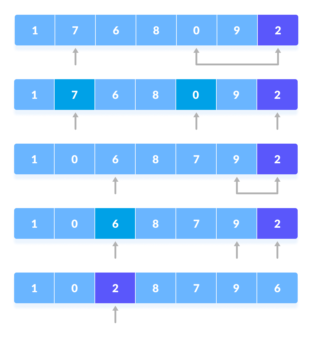
- A pointer is fixed at the pivot element. The pivot element is compared with the elements beginning from the first index.
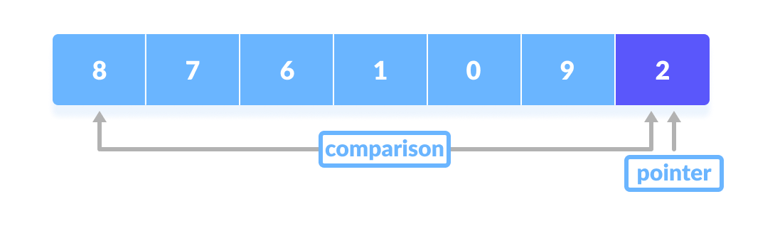
Comparison of pivot element with element beginning from the first index - If the element is greater than the pivot element, a second pointer is set for that element.
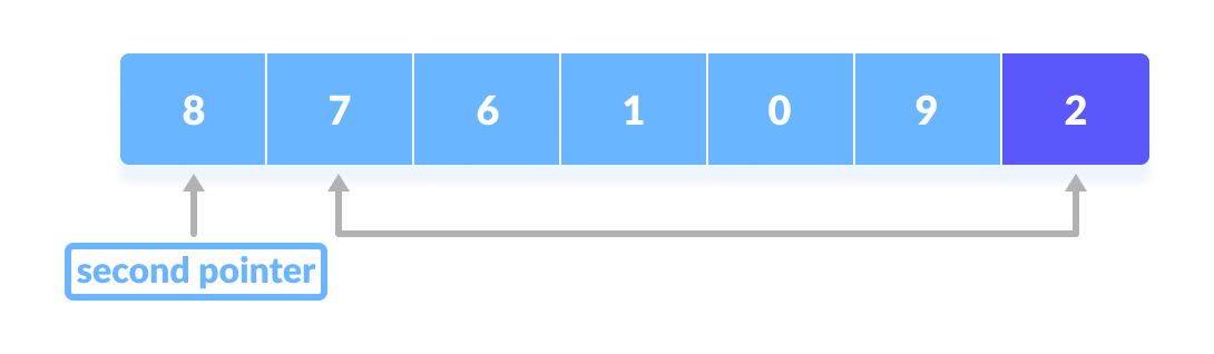
If the element is greater than the pivot element, a second pointer is set for that element. - Now, pivot is compared with other elements. If an element smaller than the pivot element is reached, the smaller element is swapped with the greater element found earlier.
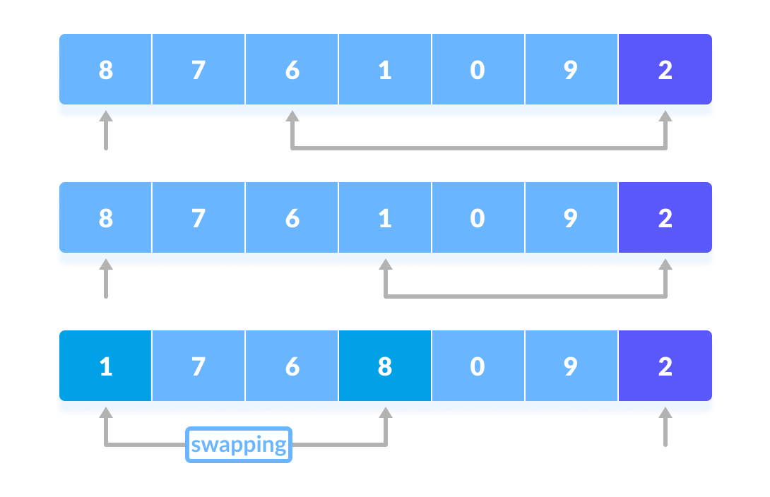
Pivot is compared with other elements. - Again, the process is repeated to set the next greater element as the second pointer. And, swap it with another smaller element.
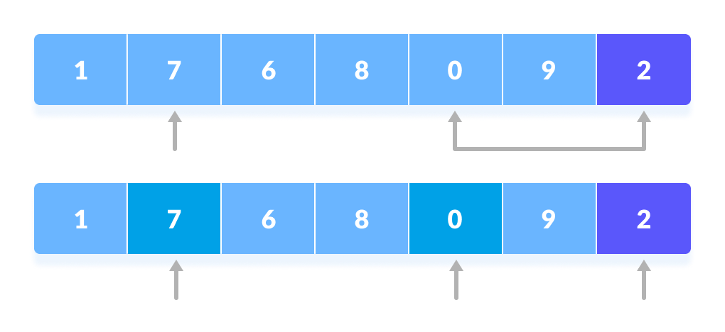
The process is repeated to set the next greater element as the second pointer. - The process goes on until the second last element is reached.
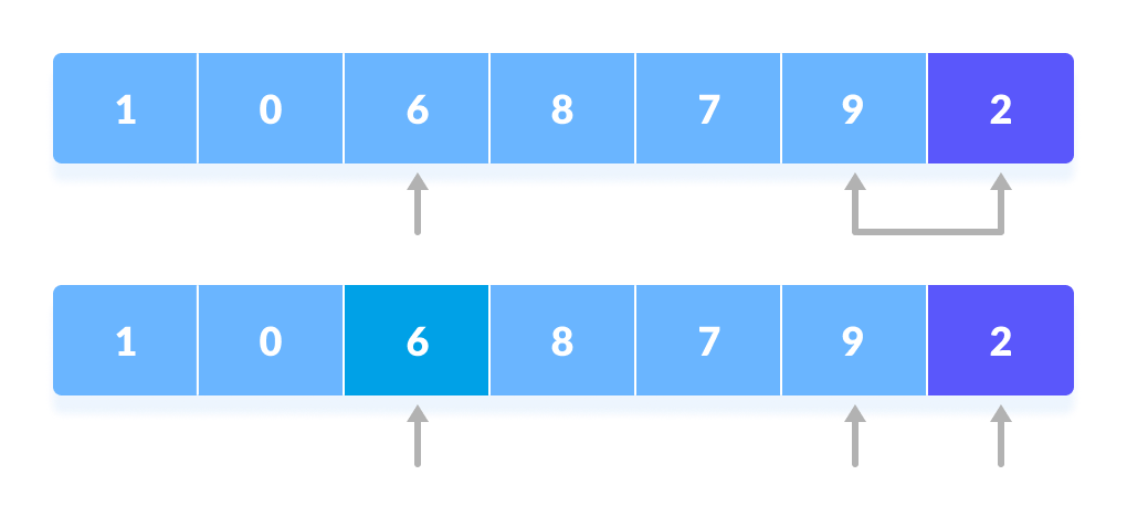
The process goes on until the second last element is reached. - Finally, the pivot element is swapped with the second pointer.
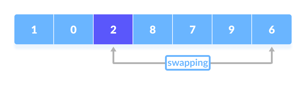
Finally, the pivot element is swapped with the second pointer.
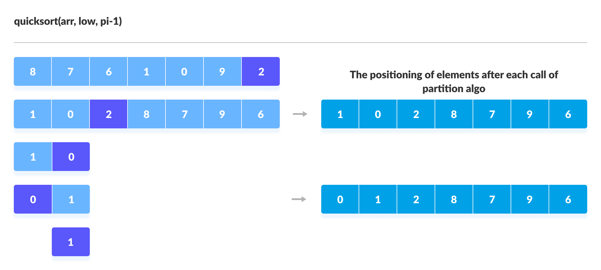
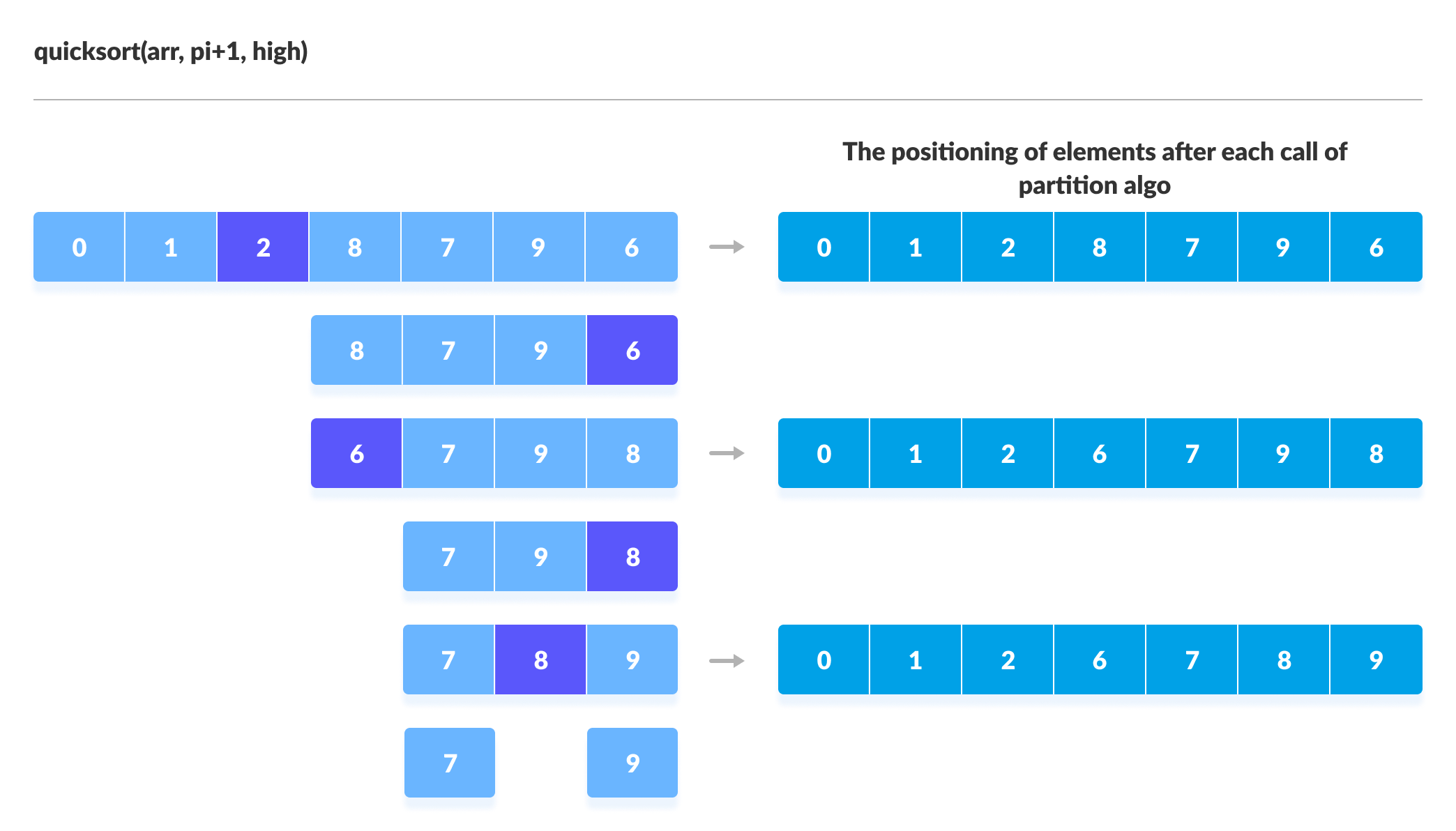
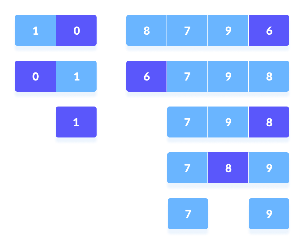
3. Divide Subarrays
Pivot elements are again chosen for the left and the right sub-parts separately. And, step 2 is repeated.
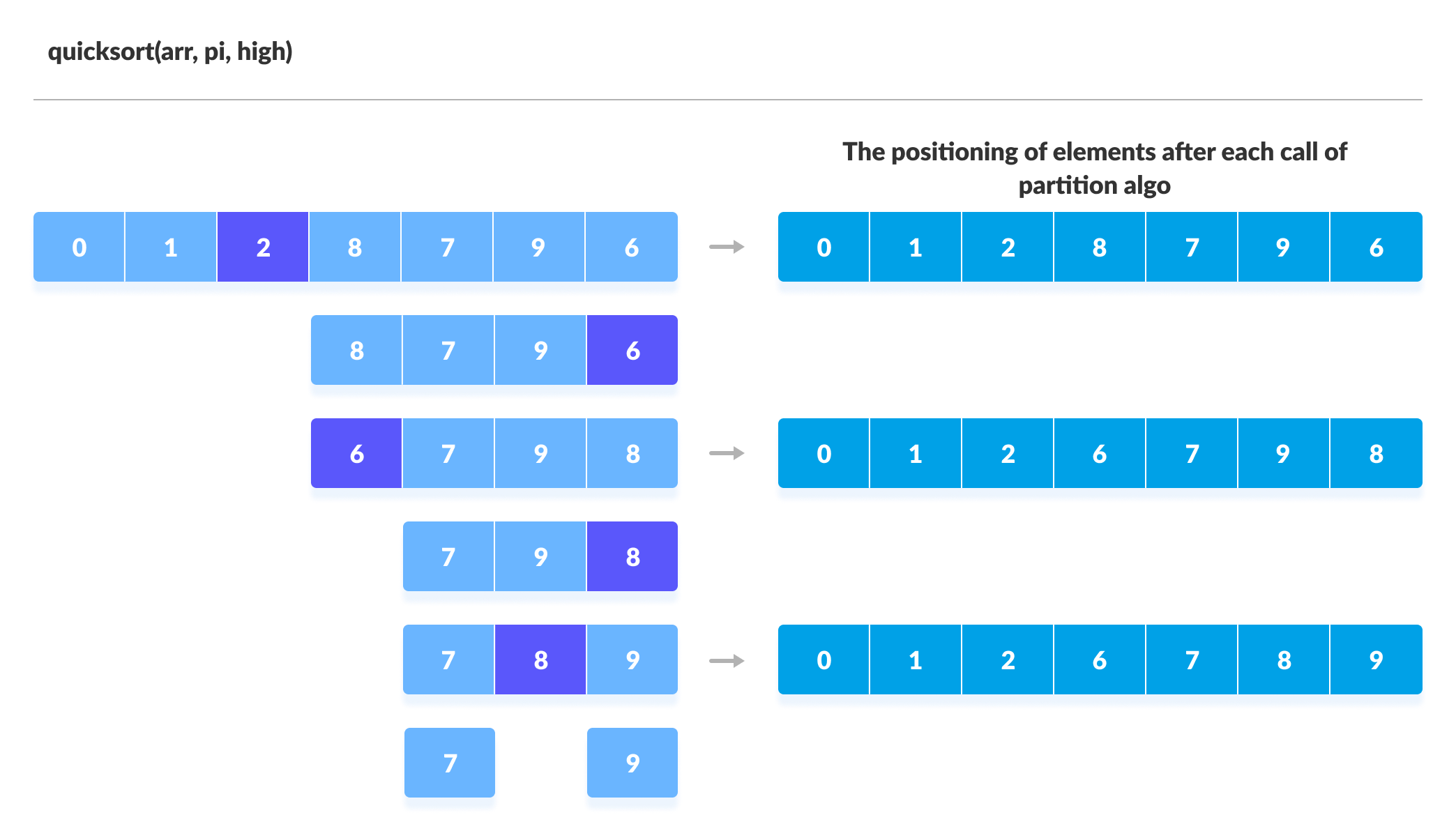
The subarrays are divided until each subarray is formed of a single element. At this point, the array is already sorted.
Quick Sort Algorithm
quickSort(array, leftmostIndex, rightmostIndex)
  if (leftmostIndex < rightmostIndex)
    pivotIndex <- partition(array,leftmostIndex, rightmostIndex)
    quickSort(array, leftmostIndex, pivotIndex - 1)
    quickSort(array, pivotIndex, rightmostIndex)

partition(array, leftmostIndex, rightmostIndex)
  set rightmostIndex as pivotIndex
  storeIndex <- leftmostIndex - 1
  for i <- leftmostIndex + 1 to rightmostIndex
  if element[i] < pivotElement
    swap element[i] and element[storeIndex]
    storeIndex++
  swap pivotElement and element[storeIndex+1]
return storeIndex + 1
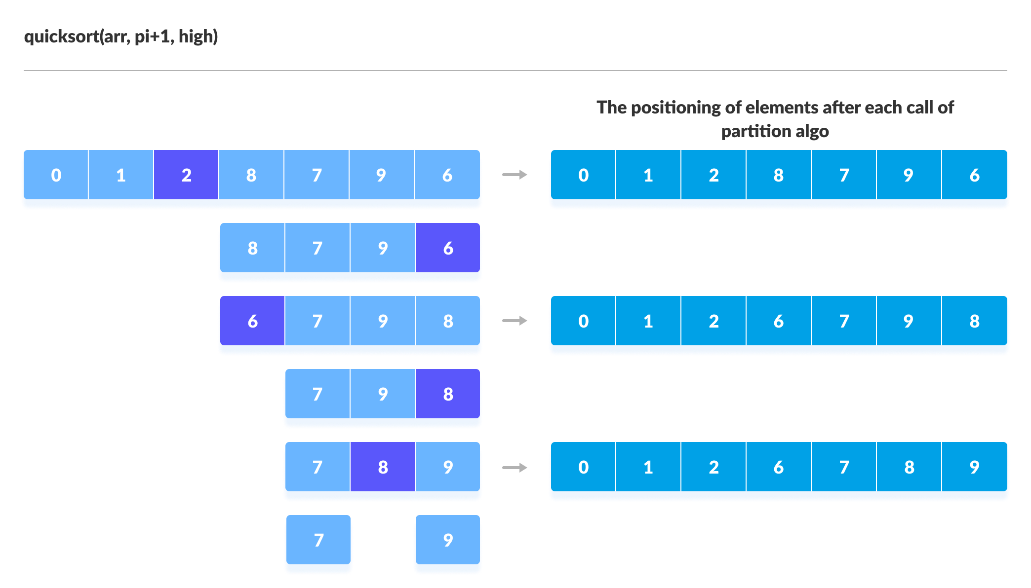
Visual Illustration of Quicksort Algorithm
You can understand the working of quicksort algorithm with the help of the illustrations below.
Quicksort Code in Python, Java, and C/C++
# Quick sort in Python

# function to find the partition position
def partition(array, low, high):

  # choose the rightmost element as pivot
  pivot = array[high]

  # pointer for greater element
  i = low - 1

  # traverse through all elements
  # compare each element with pivot
  for j in range(low, high):
    if array[j] <= pivot:
      # if element smaller than pivot is found
      # swap it with the greater element pointed by i
      i = i + 1

      # swapping element at i with element at j
      (array[i], array[j]) = (array[j], array[i])

  # swap the pivot element with the greater element specified by i
  (array[i + 1], array[high]) = (array[high], array[i + 1])

  # return the position from where partition is done
  return i + 1

# function to perform quicksort
def quickSort(array, low, high):
  if low < high:

    # find pivot element such that
    # element smaller than pivot are on the left
    # element greater than pivot are on the right
    pi = partition(array, low, high)

    # recursive call on the left of pivot
    quickSort(array, low, pi - 1)

    # recursive call on the right of pivot
    quickSort(array, pi + 1, high)


data = [8, 7, 2, 1, 0, 9, 6]
print("Unsorted Array")
print(data)

size = len(data)

quickSort(data, 0, size - 1)

print('Sorted Array in Ascending Order:')
print(data)
// Quick sort in Java

import java.util.Arrays;

class Quicksort {

  // method to find the partition position
  static int partition(int array[], int low, int high) {

    // choose the rightmost element as pivot
    int pivot = array[high];

    // pointer for greater element
    int i = (low - 1);

    // traverse through all elements
    // compare each element with pivot
    for (int j = low; j < high; j++) {
      if (array[j] <= pivot) {

        // if element smaller than pivot is found
        // swap it with the greatr element pointed by i
        i++;

        // swapping element at i with element at j
        int temp = array[i];
        array[i] = array[j];
        array[j] = temp;
      }

    }

    // swapt the pivot element with the greater element specified by i
    int temp = array[i + 1];
    array[i + 1] = array[high];
    array[high] = temp;

    // return the position from where partition is done
    return (i + 1);
  }

  static void quickSort(int array[], int low, int high) {
    if (low < high) {

      // find pivot element such that
      // elements smaller than pivot are on the left
      // elements greater than pivot are on the right
      int pi = partition(array, low, high);

      // recursive call on the left of pivot
      quickSort(array, low, pi - 1);

      // recursive call on the right of pivot
      quickSort(array, pi + 1, high);
    }
  }
}

// Main class
class Main {
  public static void main(String args[]) {

    int[] data = { 8, 7, 2, 1, 0, 9, 6 };
    System.out.println("Unsorted Array");
    System.out.println(Arrays.toString(data));

    int size = data.length;

    // call quicksort() on array data
    Quicksort.quickSort(data, 0, size - 1);

    System.out.println("Sorted Array in Ascending Order: ");
    System.out.println(Arrays.toString(data));
  }
}
// Quick sort in C

#include <stdio.h>

// function to swap elements
void swap(int *a, int *b) {
  int t = *a;
  *a = *b;
  *b = t;
}

// function to find the partition position
int partition(int array[], int low, int high) {

  // select the rightmost element as pivot
  int pivot = array[high];

  // pointer for greater element
  int i = (low - 1);

  // traverse each element of the array
  // compare them with the pivot
  for (int j = low; j < high; j++) {
    if (array[j] <= pivot) {

      // if element smaller than pivot is found
      // swap it with the greater element pointed by i
      i++;

      // swap element at i with element at j
      swap(&array[i], &array[j]);
    }
  }

  // swap the pivot element with the greater element at i
  swap(&array[i + 1], &array[high]);

  // return the partition point
  return (i + 1);
}

void quickSort(int array[], int low, int high) {
  if (low < high) {

    // find the pivot element such that
    // elements smaller than pivot are on left of pivot
    // elements greater than pivot are on right of pivot
    int pi = partition(array, low, high);

    // recursive call on the left of pivot
    quickSort(array, low, pi - 1);

    // recursive call on the right of pivot
    quickSort(array, pi + 1, high);
  }
}

// function to print array elements
void printArray(int array[], int size) {
  for (int i = 0; i < size; ++i) {
    printf("%d  ", array[i]);
  }
  printf("\n");
}

// main function
int main() {
  int data[] = {8, 7, 2, 1, 0, 9, 6};

  int n = sizeof(data) / sizeof(data[0]);

  printf("Unsorted Array\n");
  printArray(data, n);

  // perform quicksort on data
  quickSort(data, 0, n - 1);

  printf("Sorted array in ascending order: \n");
  printArray(data, n);
}
// Quick sort in C++

#include <iostream>
using namespace std;

// function to swap elements
void swap(int *a, int *b) {
  int t = *a;
  *a = *b;
  *b = t;
}

// function to print the array
void printArray(int array[], int size) {
  int i;
  for (i = 0; i < size; i++)
    cout << array[i] << " ";
  cout << endl;
}

// function to rearrange array (find the partition point)
int partition(int array[], int low, int high) {

  // select the rightmost element as pivot
  int pivot = array[high];

  // pointer for greater element
  int i = (low - 1);

  // traverse each element of the array
  // compare them with the pivot
  for (int j = low; j < high; j++) {
    if (array[j] <= pivot) {

      // if element smaller than pivot is found
      // swap it with the greater element pointed by i
      i++;

      // swap element at i with element at j
      swap(&array[i], &array[j]);
    }
  }

  // swap pivot with the greater element at i
  swap(&array[i + 1], &array[high]);

  // return the partition point
  return (i + 1);
}

void quickSort(int array[], int low, int high) {
  if (low < high) {

    // find the pivot element such that
    // elements smaller than pivot are on left of pivot
    // elements greater than pivot are on righ of pivot
    int pi = partition(array, low, high);

    // recursive call on the left of pivot
    quickSort(array, low, pi - 1);

    // recursive call on the right of pivot
    quickSort(array, pi + 1, high);
  }
}

// Driver code
int main() {
  int data[] = {8, 7, 6, 1, 0, 9, 2};
  int n = sizeof(data) / sizeof(data[0]);

  cout << "Unsorted Array: \n";
  printArray(data, n);

  // perform quicksort on data
  quickSort(data, 0, n - 1);

  cout << "Sorted array in ascending order: \n";
  printArray(data, n);
}
Quicksort Complexity
| Time Complexity | |
|---|---|
| Best | O(n*log n) |
| Worst | O(n2) |
| Average | O(n*log n) |
| Space Complexity | O(log n) |
| Stability | No |
1. Time Complexities
- Worst Case Complexity [Big-O]:
O(n2)
It occurs when the pivot element picked is either the greatest or the smallest element.
This condition leads to the case in which the pivot element lies in an extreme end of the sorted array. One sub-array is always empty and another sub-array containsn - 1elements. Thus, quicksort is called only on this sub-array.
However, the quicksort algorithm has better performance for scattered pivots.
- Best Case Complexity [Big-omega]:
O(n*log n)
It occurs when the pivot element is always the middle element or near to the middle element. - Average Case Complexity [Big-theta]:
O(n*log n)
It occurs when the above conditions do not occur.
2. Space Complexity
The space complexity for quicksort is O(log n).
Quicksort Applications
Quicksort algorithm is used when
- the programming language is good for recursion
- time complexity matters
- space complexity matters
Similar Sorting Algorithms
Merge Sort Algorithm
Merge Sort is one of the most popular sorting algorithms that is based on the principle of Divide and Conquer Algorithm.
Here, a problem is divided into multiple sub-problems. Each sub-problem is solved individually. Finally, sub-problems are combined to form the final solution.
Divide and Conquer Strategy
Using the Divide and Conquer technique, we divide a problem into subproblems. When the solution to each subproblem is ready, we 'combine' the results from the subproblems to solve the main problem.
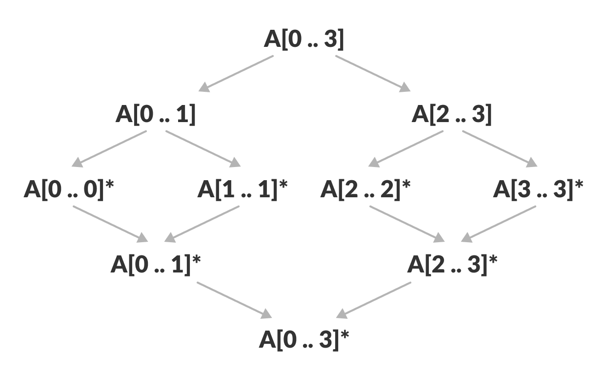
Suppose we had to sort an array A. A subproblem would be to sort a sub-section of this array starting at index p and ending at index r, denoted as A[p..r].
Divide
If q is the half-way point between p and r, then we can split the subarray A[p..r] into two arrays A[p..q] and A[q+1, r].
Conquer
In the conquer step, we try to sort both the subarrays A[p..q] and A[q+1, r]. If we haven't yet reached the base case, we again divide both these subarrays and try to sort them.
Combine
When the conquer step reaches the base step and we get two sorted subarrays A[p..q] and A[q+1, r] for array A[p..r], we combine the results by creating a sorted array A[p..r] from two sorted subarrays A[p..q] and A[q+1, r].
MergeSort Algorithm
The MergeSort function repeatedly divides the array into two halves until we reach a stage where we try to perform MergeSort on a subarray of size 1 i.e. p == r.
After that, the merge function comes into play and combines the sorted arrays into larger arrays until the whole array is merged.
MergeSort(A, p, r):
    if p > r
        return
    q = (p+r)/2
    mergeSort(A, p, q)
    mergeSort(A, q+1, r)
    merge(A, p, q, r)
To sort an entire array, we need to call
MergeSort(A, 0, length(A)-1).
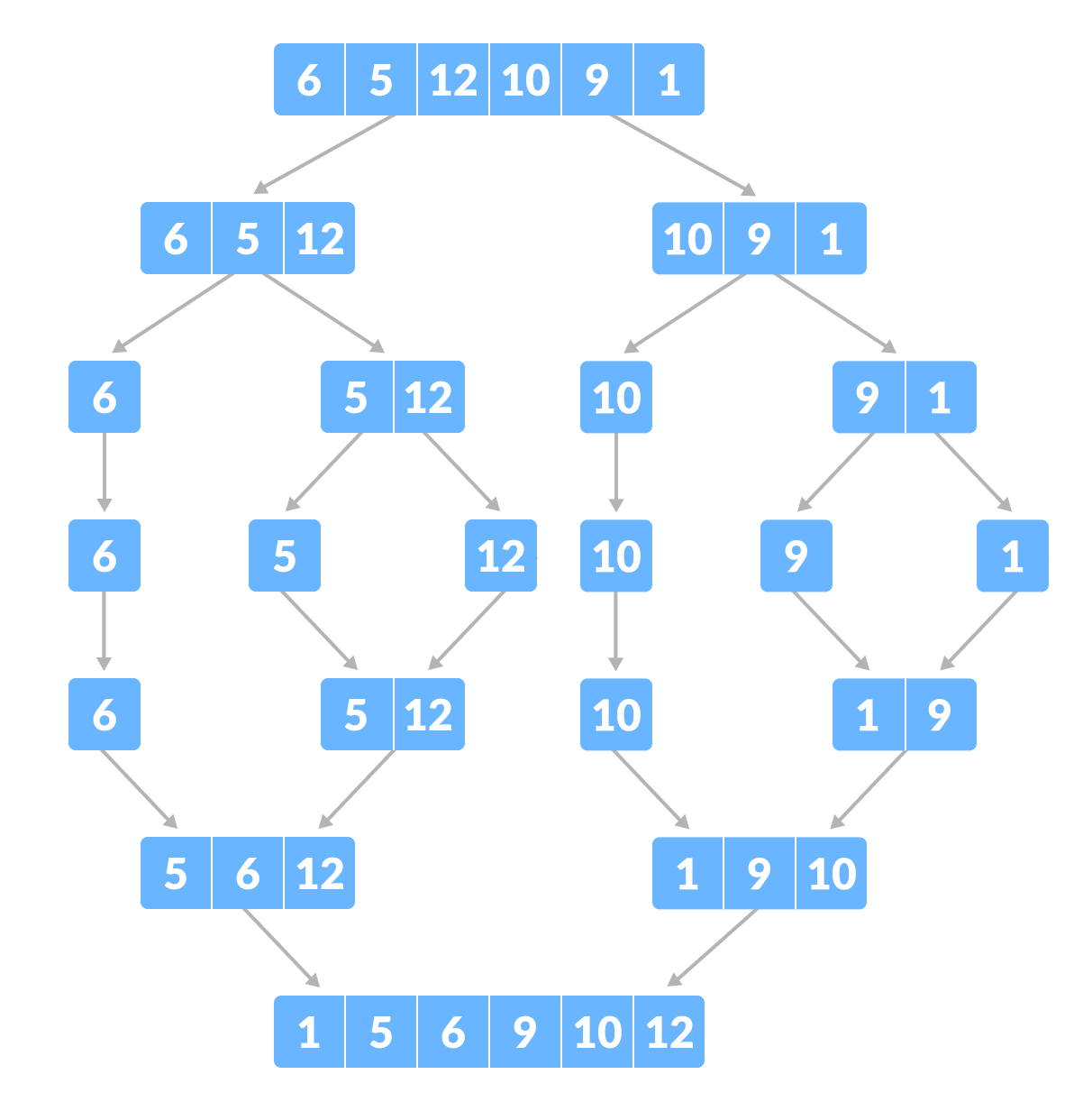
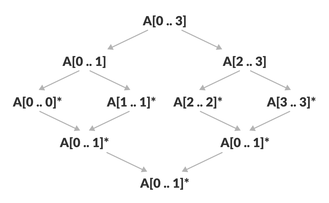
As shown in the image below, the merge sort algorithm recursively divides the array into halves until we reach the base case of array with 1 element. After that, the merge function picks up the sorted sub-arrays and merges them to gradually sort the entire array.
The merge Step of Merge Sort
Every recursive algorithm is dependent on a base case and the ability to combine the results from base cases. Merge sort is no different. The most important part of the merge sort algorithm is, you guessed it, merge step.
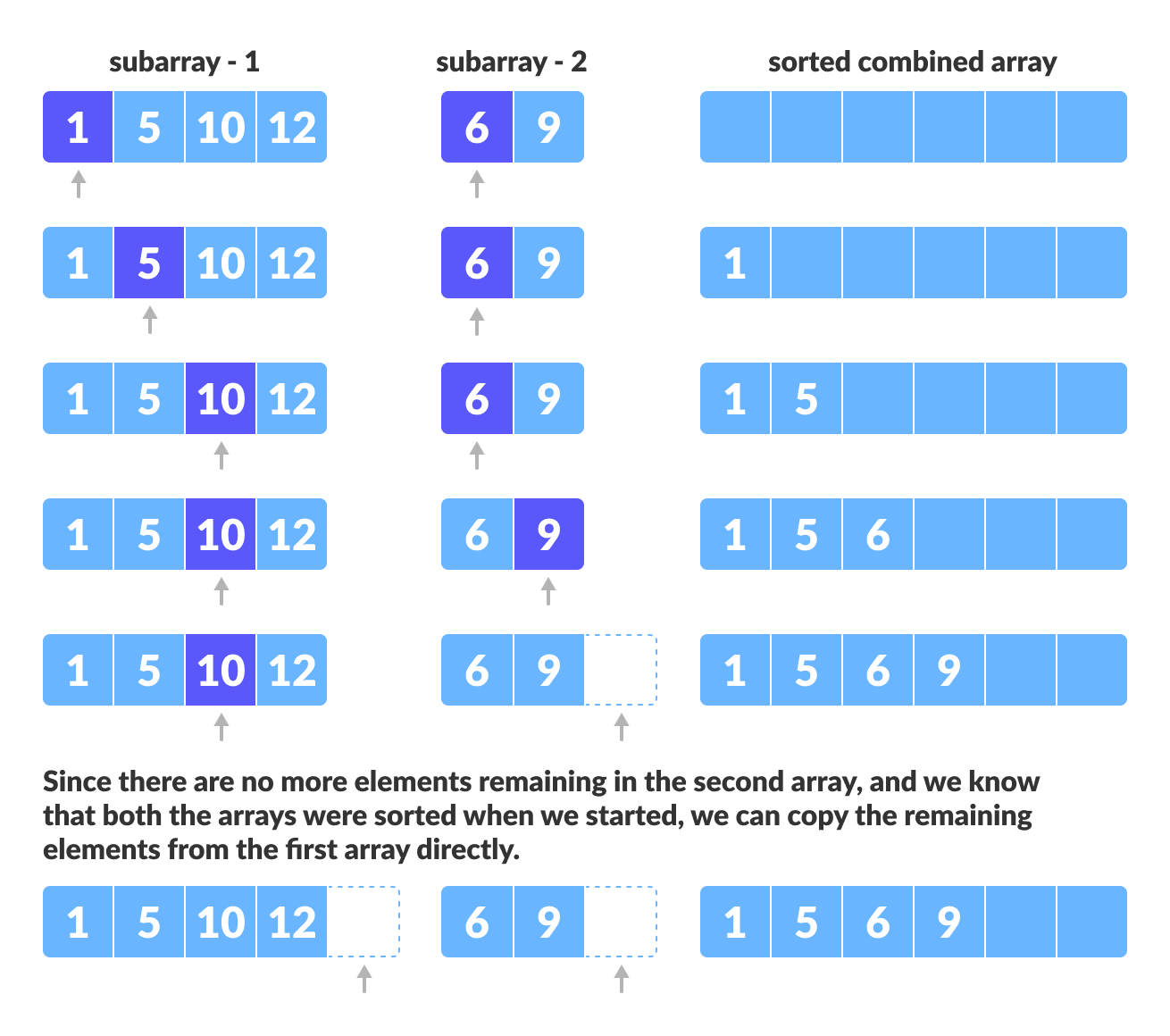
The merge step is the solution to the simple problem of merging two sorted lists(arrays) to build one large sorted list(array).
The algorithm maintains three pointers, one for each of the two arrays and one for maintaining the current index of the final sorted array.
Have we reached the end of any of the arrays?
    No:
        Compare current elements of both arrays
        Copy smaller element into sorted array
        Move pointer of element containing smaller element
    Yes:
        Copy all remaining elements of non-empty array
Writing the Code for Merge Algorithm
A noticeable difference between the merging step we described above and the one we use for merge sort is that we only perform the merge function on consecutive sub-arrays.
This is why we only need the array, the first position, the last index of the first subarray(we can calculate the first index of the second subarray) and the last index of the second subarray.
Our task is to merge two subarrays A[p..q] and A[q+1..r] to create a sorted array A[p..r]. So the inputs to the function are A, p, q and r
The merge function works as follows:
-
Create copies of the subarrays
L <- A[p..q]and M <- A[q+1..r]. -
Create three pointers i, j and k
- i maintains current index of L, starting at 1
- j maintains current index of M, starting at 1
- k maintains the current index of A[p..q], starting at p.
- Until we reach the end of either L or M, pick the larger among the elements from L and M and place them in the correct position at A[p..q]
- When we run out of elements in either L or M, pick up the remaining elements and put in A[p..q]
In code, this would look like:
// Merge two subarrays L and M into arr
void merge(int arr[], int p, int q, int r) {

    // Create L ← A[p..q] and M ← A[q+1..r]
    int n1 = q - p + 1;
    int n2 = r - q;

    int L[n1], M[n2];

    for (int i = 0; i < n1; i++)
        L[i] = arr[p + i];
    for (int j = 0; j < n2; j++)
        M[j] = arr[q + 1 + j];

    // Maintain current index of sub-arrays and main array
    int i, j, k;
    i = 0;
    j = 0;
    k = p;

    // Until we reach either end of either L or M, pick larger among
    // elements L and M and place them in the correct position at A[p..r]
    while (i < n1 && j < n2) {
        if (L[i] <= M[j]) {
            arr[k] = L[i];
            i++;
        } else {
            arr[k] = M[j];
            j++;
        }
        k++;
    }

    // When we run out of elements in either L or M,
    // pick up the remaining elements and put in A[p..r]
    while (i < n1) {
        arr[k] = L[i];
        i++;
        k++;
    }

    while (j < n2) {
        arr[k] = M[j];
        j++;
        k++;
    }
}
Merge( ) Function Explained Step-By-Step
A lot is happening in this function, so let's take an example to see how this would work.
As usual, a picture speaks a thousand words.
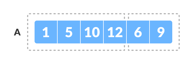
The array A[0..5] contains two sorted subarrays A[0..3] and A[4..5]. Let us see how the merge function will merge the two arrays.
void merge(int arr[], int p, int q, int r) {
// Here, p = 0, q = 4, r = 6 (size of array)
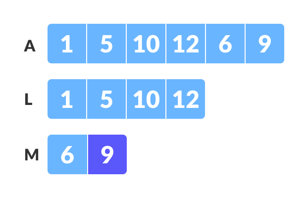
Step 1: Create duplicate copies of sub-arrays to be sorted
    // Create L ← A[p..q] and M ← A[q+1..r]
    int n1 = q - p + 1 = 3 - 0 + 1 = 4;
    int n2 = r - q = 5 - 3 = 2;

    int L[4], M[2];

    for (int i = 0; i < 4; i++)
        L[i] = arr[p + i];
        // L[0,1,2,3] = A[0,1,2,3] = [1,5,10,12]

    for (int j = 0; j < 2; j++)
        M[j] = arr[q + 1 + j];
        // M[0,1] = A[4,5] = [6,9]
Step 2: Maintain current index of sub-arrays and main array
    int i, j, k;
    i = 0;
    j = 0;
    k = p;
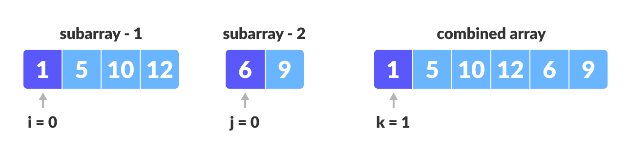
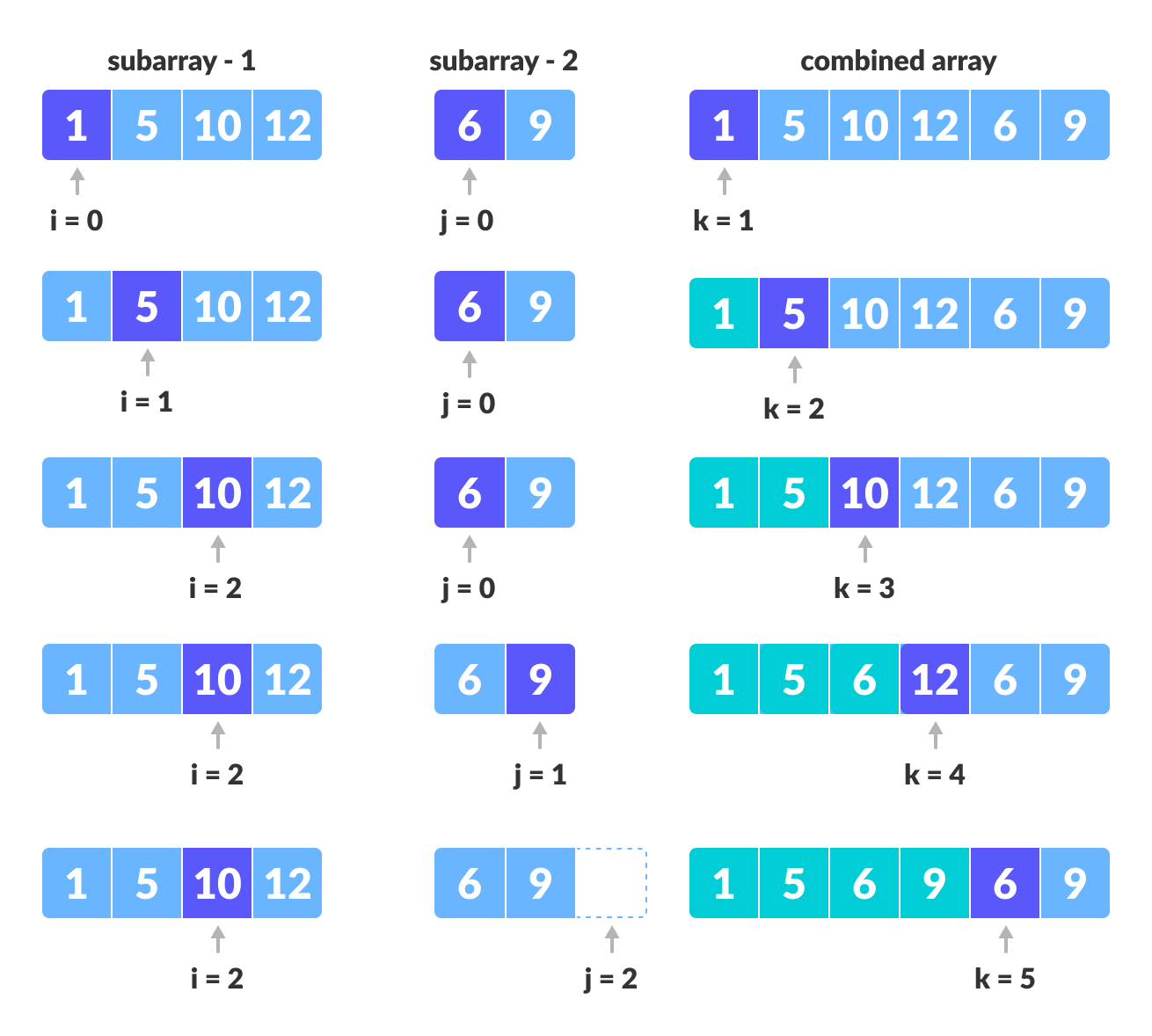
Step 3: Until we reach the end of either L or M, pick larger among elements L and M and place them in the correct position at A[p..r]
    while (i < n1 && j < n2) {
        if (L[i] <= M[j]) {
            arr[k] = L[i]; i++;
        }
        else {
            arr[k] = M[j];
            j++;
        }
        k++;
    }
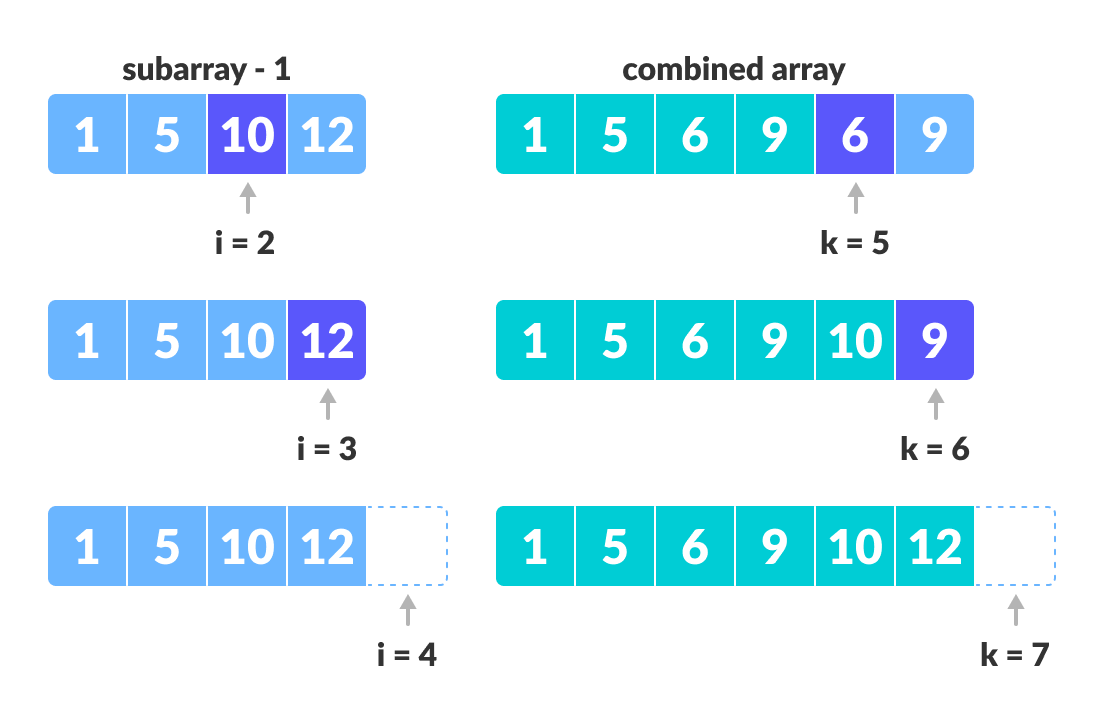
Step 4: When we run out of elements in either L or M, pick up the remaining elements and put in A[p..r]
    // We exited the earlier loop because j < n2 doesn't hold
    while (i < n1)
    {
        arr[k] = L[i];
        i++;
        k++;
    }
    // We exited the earlier loop because i < n1 doesn't hold
    while (j < n2)
    {
        arr[k] = M[j];
        j++;
        k++;
    }
}
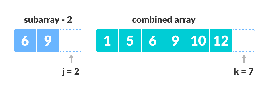
This step would have been needed if the size of M was greater than L.
At the end of the merge function, the subarray A[p..r] is sorted.
Merge Sort Code in Python, Java, and C/C++
Merge Sort Visualization: Don't just read about merge sort, watch it happen live. See how each line of the algorithm works step-by-step with our new DSA visualizer. Try it yourself!
# MergeSort in Python


def mergeSort(array):
    if len(array) > 1:

        #  r is the point where the array is divided into two subarrays
        r = len(array)//2
        L = array[:r]
        M = array[r:]

        # Sort the two halves
        mergeSort(L)
        mergeSort(M)

        i = j = k = 0

        # Until we reach either end of either L or M, pick larger among
        # elements L and M and place them in the correct position at A[p..r]
        while i < len(L) and j < len(M):
            if L[i] < M[j]:
                array[k] = L[i]
                i += 1
            else:
                array[k] = M[j]
                j += 1
            k += 1

        # When we run out of elements in either L or M,
        # pick up the remaining elements and put in A[p..r]
        while i < len(L):
            array[k] = L[i]
            i += 1
            k += 1

        while j < len(M):
            array[k] = M[j]
            j += 1
            k += 1


# Print the array
def printList(array):
    for i in range(len(array)):
        print(array[i], end=" ")
    print()


# Driver program
if __name__ == '__main__':
    array = [6, 5, 12, 10, 9, 1]

    mergeSort(array)

    print("Sorted array is: ")
    printList(array)
// Merge sort in Java

class MergeSort {

  // Merge two subarrays L and M into arr
  void merge(int arr[], int p, int q, int r) {

    int n1 = q - p + 1;
    int n2 = r - q;

    int L[] = new int[n1];
    int M[] = new int[n2];

    for (int i = 0; i < n1; i++)
      L[i] = arr[p + i];
    for (int j = 0; j < n2; j++)
      M[j] = arr[q + 1 + j];

    // Maintain current index of sub-arrays and main array
    int i, j, k;
    i = 0;
    j = 0;
    k = p;

    // Until we reach either end of either L or M, pick larger among
    // elements L and M and place them in the correct position at A[p..r]
    while (i < n1 && j < n2) {
      if (L[i] <= M[j]) {
        arr[k] = L[i];
        i++;
      } else {
        arr[k] = M[j];
        j++;
      }
      k++;
    }

    // When we run out of elements in either L or M,
    // pick up the remaining elements and put in A[p..r]
    while (i < n1) {
      arr[k] = L[i];
      i++;
      k++;
    }

    while (j < n2) {
      arr[k] = M[j];
      j++;
      k++;
    }
  }

  // Divide the array into two subarrays, sort them and merge them
  void mergeSort(int arr[], int l, int r) {
    if (l < r) {

      // m is the point where the array is divided into two subarrays
      int m = (l + r) / 2;

      mergeSort(arr, l, m);
      mergeSort(arr, m + 1, r);

      // Merge the sorted subarrays
      merge(arr, l, m, r);
    }
  }

  // Print the array
  static void printArray(int arr[]) {
    int n = arr.length;
    for (int i = 0; i < n; ++i)
      System.out.print(arr[i] + " ");
    System.out.println();
  }

  // Driver program
  public static void main(String args[]) {
    int arr[] = { 6, 5, 12, 10, 9, 1 };

    MergeSort ob = new MergeSort();
    ob.mergeSort(arr, 0, arr.length - 1);

    System.out.println("Sorted array:");
    printArray(arr);
  }
}
// Merge sort in C

#include <stdio.h>

// Merge two subarrays L and M into arr
void merge(int arr[], int p, int q, int r) {

  // Create L ← A[p..q] and M ← A[q+1..r]
  int n1 = q - p + 1;
  int n2 = r - q;

  int L[n1], M[n2];

  for (int i = 0; i < n1; i++)
    L[i] = arr[p + i];
  for (int j = 0; j < n2; j++)
    M[j] = arr[q + 1 + j];

  // Maintain current index of sub-arrays and main array
  int i, j, k;
  i = 0;
  j = 0;
  k = p;

  // Until we reach either end of either L or M, pick larger among
  // elements L and M and place them in the correct position at A[p..r]
  while (i < n1 && j < n2) {
    if (L[i] <= M[j]) {
      arr[k] = L[i];
      i++;
    } else {
      arr[k] = M[j];
      j++;
    }
    k++;
  }

  // When we run out of elements in either L or M,
  // pick up the remaining elements and put in A[p..r]
  while (i < n1) {
    arr[k] = L[i];
    i++;
    k++;
  }

  while (j < n2) {
    arr[k] = M[j];
    j++;
    k++;
  }
}

// Divide the array into two subarrays, sort them and merge them
void mergeSort(int arr[], int l, int r) {
  if (l < r) {

    // m is the point where the array is divided into two subarrays
    int m = l + (r - l) / 2;

    mergeSort(arr, l, m);
    mergeSort(arr, m + 1, r);

    // Merge the sorted subarrays
    merge(arr, l, m, r);
  }
}

// Print the array
void printArray(int arr[], int size) {
  for (int i = 0; i < size; i++)
    printf("%d ", arr[i]);
  printf("\n");
}

// Driver program
int main() {
  int arr[] = {6, 5, 12, 10, 9, 1};
  int size = sizeof(arr) / sizeof(arr[0]);

  mergeSort(arr, 0, size - 1);

  printf("Sorted array: \n");
  printArray(arr, size);
}
// Merge sort in C++
#include <iostream>
#include <vector>
using namespace std;

// Merge two subarrays L and M into arr
void merge(int arr[], int p, int q, int r) {

  // Create L ← A[p..q] and M ← A[q+1..r]
  int n1 = q - p + 1;
  int n2 = r - q;

  // Use std::vector to dynamically allocate arrays
  vector<int> L(n1);
  vector<int> M(n2);

  for (int i = 0; i < n1; i++)
    L[i] = arr[p + i];

  for (int j = 0; j < n2; j++)
    M[j] = arr[q + 1 + j];

  // Maintain current index of sub-arrays and main array
  int i = 0, j = 0, k = p;

  // Until we reach either end of either L or M, pick larger among
  // elements L and M and place them in the correct position at A[p..r]
  while (i < n1 && j < n2) {
    if (L[i] <= M[j]) {
      arr[k] = L[i];
      i++;
    } else {
      arr[k] = M[j];
      j++;
    }
    k++;
  }

  // When we run out of elements in either L or M,
  // pick up the remaining elements and put in A[p..r]
  while (i < n1) {
    arr[k] = L[i];
    i++;
    k++;
  }

  while (j < n2) {
    arr[k] = M[j];
    j++;
    k++;
  }
}

// Divide the array into two subarrays, sort them and merge them
void mergeSort(int arr[], int l, int r) {
  if (l < r) {
    // m is the point where the array is divided into two subarrays
    int m = l + (r - l) / 2;

    mergeSort(arr, l, m);
    mergeSort(arr, m + 1, r);
    // Merge the sorted subarrays
    merge(arr, l, m, r);
  }
}

// Print the array
void printArray(int arr[], int size) {
  for (int i = 0; i < size; i++)
    cout << arr[i] << " ";
  cout << endl;
}

// Driver program
int main() {
  int arr[] = {6, 5, 12, 10, 9, 1};
  int size = sizeof(arr) / sizeof(arr[0]);
  mergeSort(arr, 0, size - 1);
  cout << "Sorted array: \n";
  printArray(arr, size);
  return 0;
}
Merge Sort Complexity
| Time Complexity | |
|---|---|
| Best | O(n*log n) |
| Worst | O(n*log n) |
| Average | O(n*log n) |
| Space Complexity | O(n) |
| Stability | Yes |
Time Complexity
Best Case Complexity: O(n*log n)
Worst Case Complexity: O(n*log n)
Average Case Complexity: O(n*log n)
Space Complexity
The space complexity of merge sort is O(n).
Merge Sort Applications
- Inversion count problem
- External sorting
- E-commerce applications
Similar Sorting Algorithms
Heap Sort Algorithm
Heap Sort is a popular and efficient sorting algorithm in computer programming. Learning how to write the heap sort algorithm requires knowledge of two types of data structures - arrays and trees.
The initial set of numbers that we want to sort is stored in an array e.g. [10, 3, 76, 34, 23, 32] and after sorting, we get a sorted array [3,10,23,32,34,76].
Heap sort works by visualizing the elements of the array as a special kind of complete binary tree called a heap.
Note: As a prerequisite, you must know about a complete binary tree and heap data structure.
Relationship between Array Indexes and Tree Elements
A complete binary tree has an interesting property that we can use to find the children and parents of any node.
If the index of any element in the array is i, the element in the index 2i+1 will become the left child and element in 2i+2 index will become the right child. Also, the parent of any element at index i is given by the lower bound of (i-1)/2.
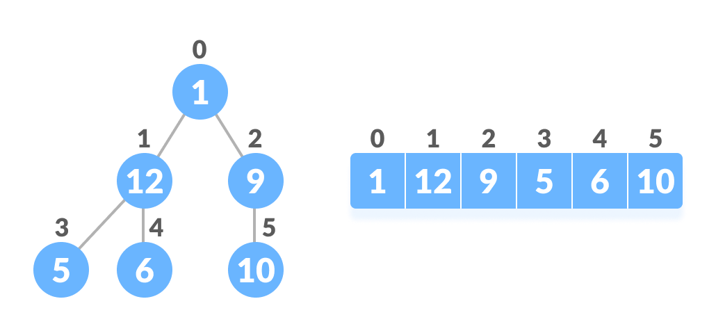
Let's test it out,
Left child of 1 (index 0)
= element in (2*0+1) index
= element in 1 index
= 12


Right child of 1
= element in (2*0+2) index
= element in 2 index
= 9

Similarly,
Left child of 12 (index 1)
= element in (2*1+1) index
= element in 3 index
= 5

Right child of 12
= element in (2*1+2) index
= element in 4 index
= 6
Let us also confirm that the rules hold for finding parent of any node
Parent of 9 (position 2)
= (2-1)/2
= ½
= 0.5
~ 0 index
= 1

Parent of 12 (position 1)
= (1-1)/2
= 0 index
= 1
Understanding this mapping of array indexes to tree positions is critical to understanding how the Heap Data Structure works and how it is used to implement Heap Sort.
What is Heap Data Structure?
Heap is a special tree-based data structure. A binary tree is said to follow a heap data structure if
- it is a complete binary tree
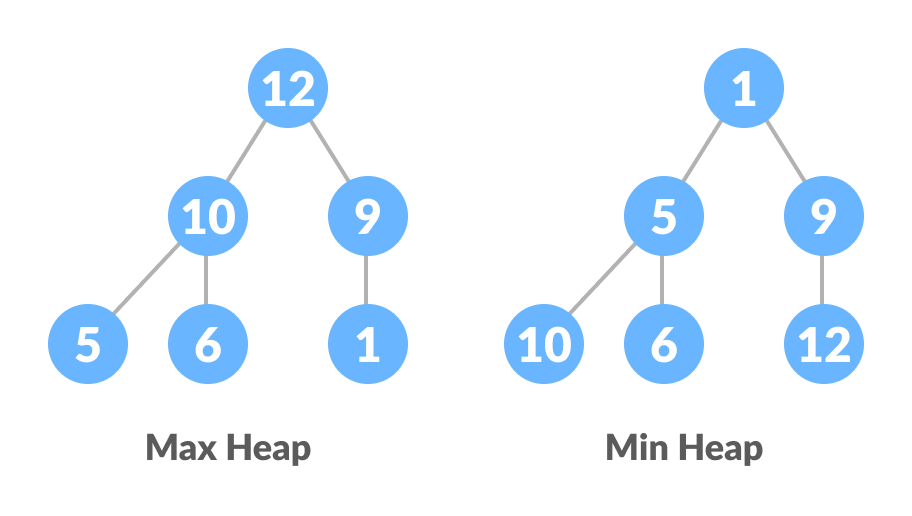
- All nodes in the tree follow the property that they are greater than their children i.e. the largest element is at the root and both its children and smaller than the root and so on. Such a heap is called a max-heap. If instead, all nodes are smaller than their children, it is called a min-heap
The following example diagram shows Max-Heap and Min-Heap.
To learn more about it, please visit Heap Data Structure.
How to "heapify" a tree
Starting from a complete binary tree, we can modify it to become a Max-Heap by running a function called heapify on all the non-leaf elements of the heap.
Since heapify uses recursion, it can be difficult to grasp. So let's first think about how you would heapify a tree with just three elements.
heapify(array)
    Root = array[0]
    Largest = largest( array[0] , array [2*0 + 1]. array[2*0+2])
    if(Root != Largest)
          Swap(Root, Largest)
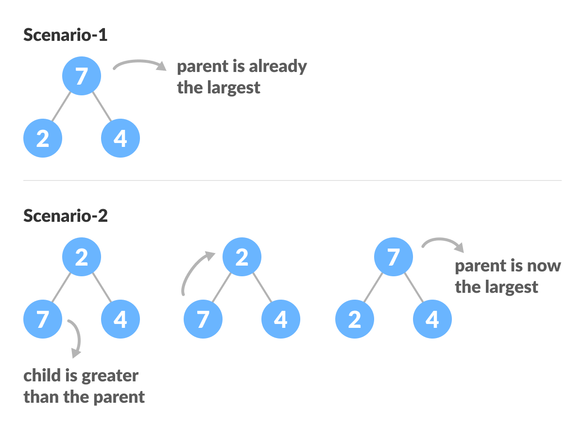
The example above shows two scenarios - one in which the root is the largest element and we don't need to do anything. And another in which the root had a larger element as a child and we needed to swap to maintain max-heap property.
If you're worked with recursive algorithms before, you've probably identified that this must be the base case.
Now let's think of another scenario in which there is more than one level.
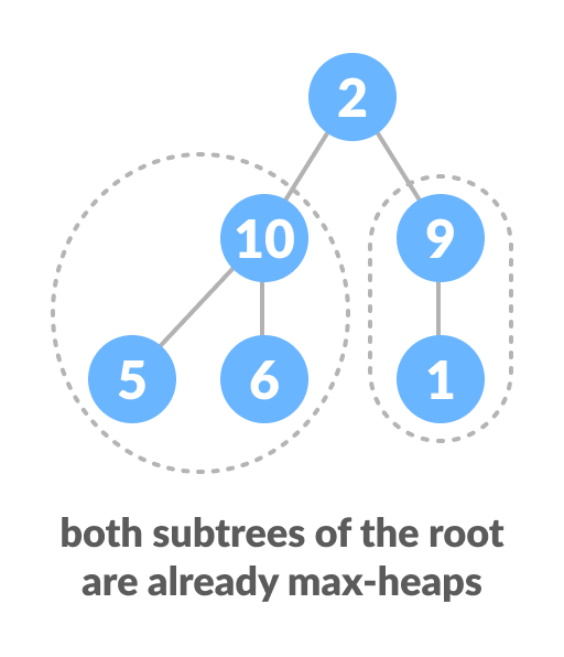
The top element isn't a max-heap but all the sub-trees are max-heaps.
To maintain the max-heap property for the entire tree, we will have to keep pushing 2 downwards until it reaches its correct position.
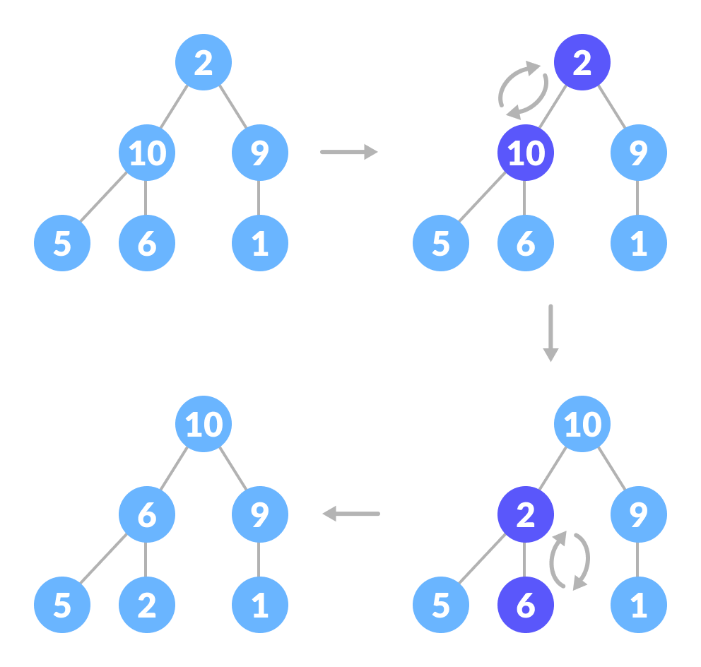
Thus, to maintain the max-heap property in a tree where both sub-trees are max-heaps, we need to run heapify on the root element repeatedly until it is larger than its children or it becomes a leaf node.
We can combine both these conditions in one heapify function as
void heapify(int arr[], int n, int i) {
  // Find largest among root, left child and right child
  int largest = i;
  int left = 2 * i + 1;
  int right = 2 * i + 2;

  if (left < n && arr[left] > arr[largest])
    largest = left;

  if (right < n && arr[right] > arr[largest])
    largest = right;

    // Swap and continue heapifying if root is not largest
    if (largest != i) {
      swap(&arr[i], &arr[largest]);
      heapify(arr, n, largest);
  }
}
This function works for both the base case and for a tree of any size. We can thus move the root element to the correct position to maintain the max-heap status for any tree size as long as the sub-trees are max-heaps.
Build max-heap
To build a max-heap from any tree, we can thus start heapifying each sub-tree from the bottom up and end up with a max-heap after the function is applied to all the elements including the root element.
In the case of a complete tree, the first index of a non-leaf node is given by n/2 - 1. All other nodes after that are leaf-nodes and thus don't need to be heapified.
So, we can build a maximum heap as
    // Build heap (rearrange array)
    for (int i = n / 2 - 1; i >= 0; i--)
      heapify(arr, n, i);
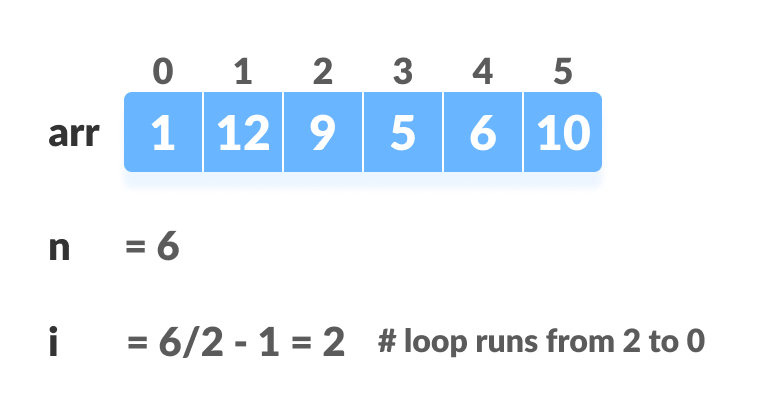
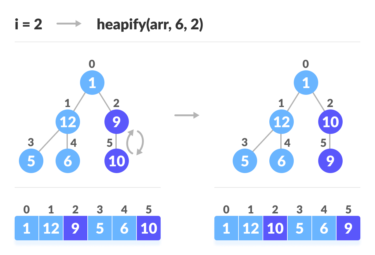
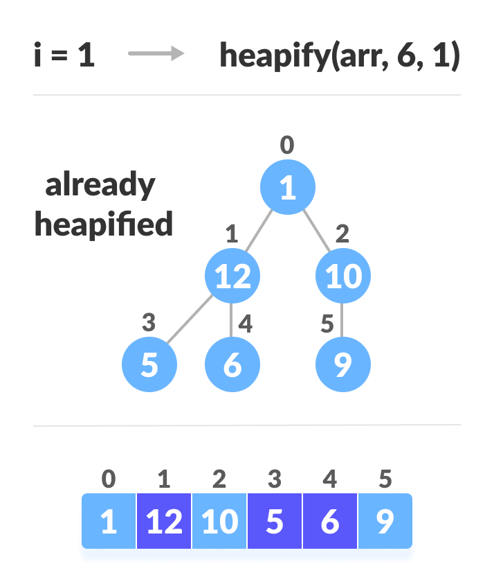
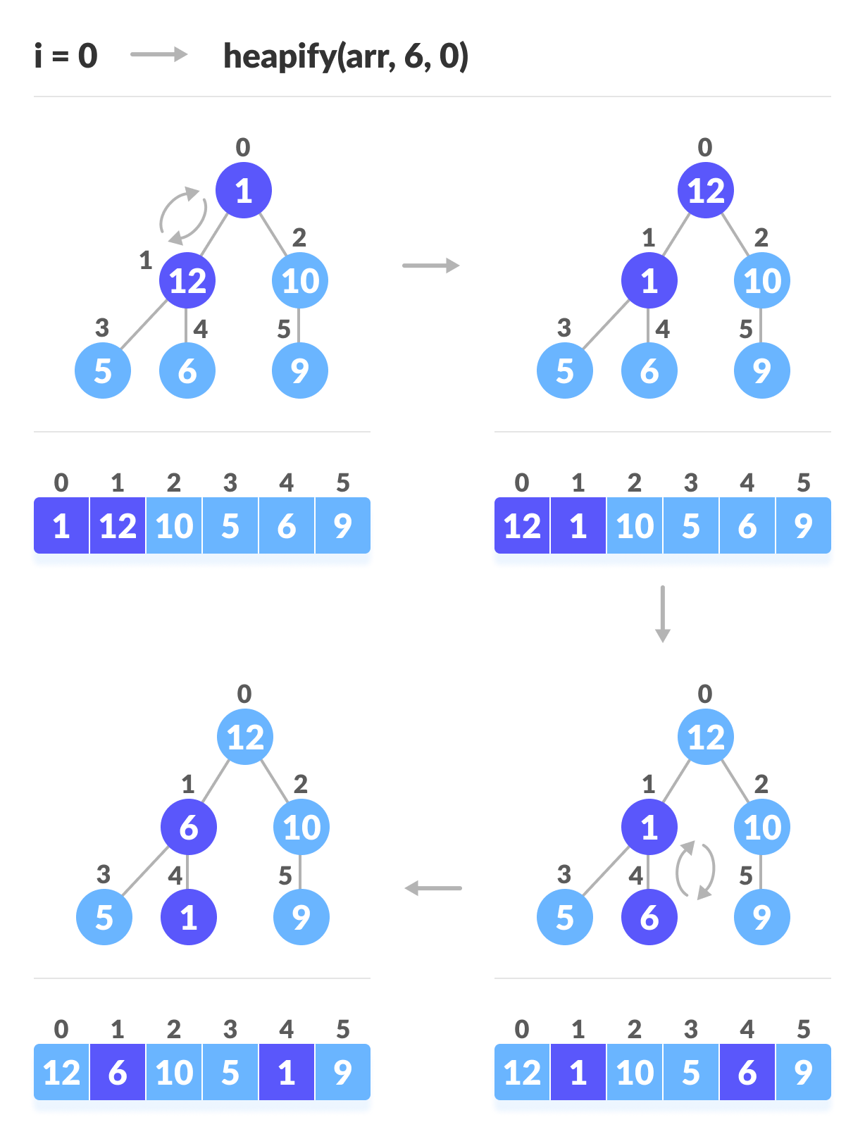
As shown in the above diagram, we start by heapifying the lowest smallest trees and gradually move up until we reach the root element.
If you've understood everything till here, congratulations, you are on your way to mastering the Heap sort.
Working of Heap Sort
- Since the tree satisfies Max-Heap property, then the largest item is stored at the root node.
- Swap: Remove the root element and put at the end of the array (nth position) Put the last item of the tree (heap) at the vacant place.
- Remove: Reduce the size of the heap by 1.
- Heapify: Heapify the root element again so that we have the highest element at root.
- The process is repeated until all the items of the list are sorted.
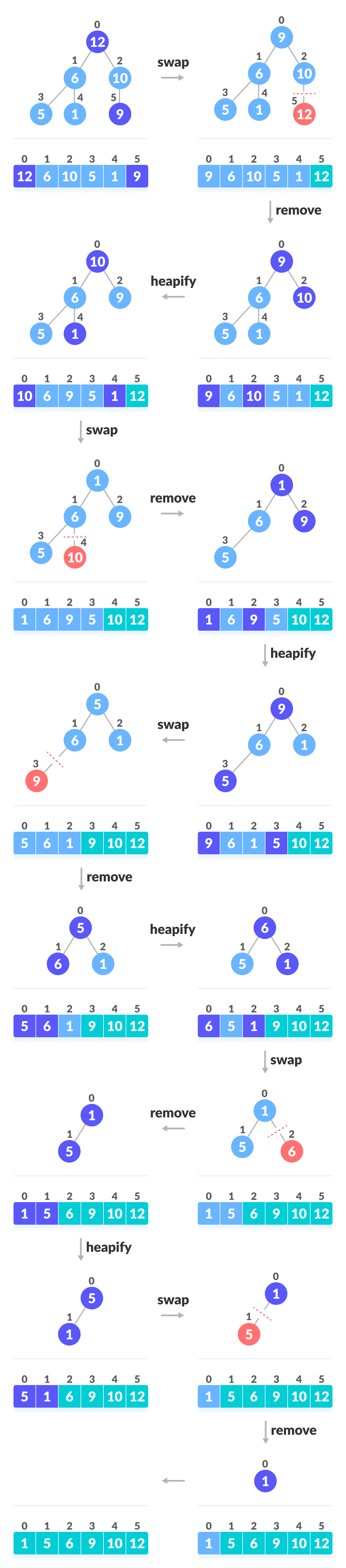
The code below shows the operation.
    // Heap sort
    for (int i = n - 1; i >= 0; i--) {
      swap(&arr[0], &arr[i]);

      // Heapify root element to get highest element at root again
      heapify(arr, i, 0);
    }
Heap Sort Code in Python, Java, and C/C++
# Heap Sort in python


  def heapify(arr, n, i):
      # Find largest among root and children
      largest = i
      l = 2 * i + 1
      r = 2 * i + 2

      if l < n and arr[i] < arr[l]:
          largest = l

      if r < n and arr[largest] < arr[r]:
          largest = r

      # If root is not largest, swap with largest and continue heapifying
      if largest != i:
          arr[i], arr[largest] = arr[largest], arr[i]
          heapify(arr, n, largest)


  def heapSort(arr):
      n = len(arr)

      # Build max heap
      for i in range(n//2, -1, -1):
          heapify(arr, n, i)

      for i in range(n-1, 0, -1):
          # Swap
          arr[i], arr[0] = arr[0], arr[i]

          # Heapify root element
          heapify(arr, i, 0)


  arr = [1, 12, 9, 5, 6, 10]
  heapSort(arr)
  n = len(arr)
  print("Sorted array is")
  for i in range(n):
      print("%d " % arr[i], end='')
// Heap Sort in Java

  public class HeapSort {

    public void sort(int arr[]) {
      int n = arr.length;

      // Build max heap
      for (int i = n / 2 - 1; i >= 0; i--) {
        heapify(arr, n, i);
      }

      // Heap sort
      for (int i = n - 1; i >= 0; i--) {
        int temp = arr[0];
        arr[0] = arr[i];
        arr[i] = temp;

        // Heapify root element
        heapify(arr, i, 0);
      }
    }

    void heapify(int arr[], int n, int i) {
      // Find largest among root, left child and right child
      int largest = i;
      int l = 2 * i + 1;
      int r = 2 * i + 2;

      if (l < n && arr[l] > arr[largest])
        largest = l;

      if (r < n && arr[r] > arr[largest])
        largest = r;

      // Swap and continue heapifying if root is not largest
      if (largest != i) {
        int swap = arr[i];
        arr[i] = arr[largest];
        arr[largest] = swap;

        heapify(arr, n, largest);
      }
    }

    // Function to print an array
    static void printArray(int arr[]) {
      int n = arr.length;
      for (int i = 0; i < n; ++i)
        System.out.print(arr[i] + " ");
      System.out.println();
    }

    // Driver code
    public static void main(String args[]) {
      int arr[] = { 1, 12, 9, 5, 6, 10 };

      HeapSort hs = new HeapSort();
      hs.sort(arr);

      System.out.println("Sorted array is");
      printArray(arr);
    }
  }
// Heap Sort in C

  #include <stdio.h>

  // Function to swap the the position of two elements
  void swap(int *a, int *b) {
    int temp = *a;
    *a = *b;
    *b = temp;
  }

  void heapify(int arr[], int n, int i) {
    // Find largest among root, left child and right child
    int largest = i;
    int left = 2 * i + 1;
    int right = 2 * i + 2;

    if (left < n && arr[left] > arr[largest])
      largest = left;

    if (right < n && arr[right] > arr[largest])
      largest = right;

    // Swap and continue heapifying if root is not largest
    if (largest != i) {
      swap(&arr[i], &arr[largest]);
      heapify(arr, n, largest);
    }
  }

  // Main function to do heap sort
  void heapSort(int arr[], int n) {
    // Build max heap
    for (int i = n / 2 - 1; i >= 0; i--)
      heapify(arr, n, i);

    // Heap sort
    for (int i = n - 1; i >= 0; i--) {
      swap(&arr[0], &arr[i]);

      // Heapify root element to get highest element at root again
      heapify(arr, i, 0);
    }
  }

  // Print an array
  void printArray(int arr[], int n) {
    for (int i = 0; i < n; ++i)
      printf("%d ", arr[i]);
    printf("\n");
  }

  // Driver code
  int main() {
    int arr[] = {1, 12, 9, 5, 6, 10};
    int n = sizeof(arr) / sizeof(arr[0]);

    heapSort(arr, n);

    printf("Sorted array is \n");
    printArray(arr, n);
  }
// Heap Sort in C++

  #include <iostream>
  using namespace std;

  void heapify(int arr[], int n, int i) {
    // Find largest among root, left child and right child
    int largest = i;
    int left = 2 * i + 1;
    int right = 2 * i + 2;

    if (left < n && arr[left] > arr[largest])
      largest = left;

    if (right < n && arr[right] > arr[largest])
      largest = right;

    // Swap and continue heapifying if root is not largest
    if (largest != i) {
      swap(arr[i], arr[largest]);
      heapify(arr, n, largest);
    }
  }

  // main function to do heap sort
  void heapSort(int arr[], int n) {
    // Build max heap
    for (int i = n / 2 - 1; i >= 0; i--)
      heapify(arr, n, i);

    // Heap sort
    for (int i = n - 1; i >= 0; i--) {
      swap(arr[0], arr[i]);

      // Heapify root element to get highest element at root again
      heapify(arr, i, 0);
    }
  }

  // Print an array
  void printArray(int arr[], int n) {
    for (int i = 0; i < n; ++i)
      cout << arr[i] << " ";
    cout << "\n";
  }

  // Driver code
  int main() {
    int arr[] = {1, 12, 9, 5, 6, 10};
    int n = sizeof(arr) / sizeof(arr[0]);
    heapSort(arr, n);

    cout << "Sorted array is \n";
    printArray(arr, n);
  }
Heap Sort Complexity
| Time Complexity | |
|---|---|
| Best | O(nlog n) |
| Worst | O(nlog n) |
| Average | O(nlog n) |
| Space Complexity | O(1) |
| Stability | No |
Heap Sort has O(nlog n) time complexities for all the cases ( best case, average case, and worst case).
Let us understand the reason why. The height of a complete binary tree containing n elements is log n
As we have seen earlier, to fully heapify an element whose subtrees are already max-heaps, we need to keep comparing the element with its left and right children and pushing it downwards until it reaches a point where both its children are smaller than it.
In the worst case scenario, we will need to move an element from the root to the leaf node making a multiple of log(n) comparisons and swaps.
During the build_max_heap stage, we do that for n/2 elements so the worst case complexity of the build_heap step is n/2*log n ~ nlog n.
During the sorting step, we exchange the root element with the last element and heapify the root element. For each element, this again takes log n worst time because we might have to bring the element all the way from the root to the leaf. Since we repeat this n times, the heap_sort step is also nlog n.
Also since the build_max_heap and heap_sort steps are executed one after another, the algorithmic complexity is not multiplied and it remains in the order of nlog n.
Also it performs sorting in O(1) space complexity. Compared with Quick Sort, it has a better worst case ( O(nlog n) ). Quick Sort has complexity O(n^2) for worst case. But in other cases, Quick Sort is fast. Introsort is an alternative to heapsort that combines quicksort and heapsort to retain advantages of both: worst case speed of heapsort and average speed of quicksort.
Heap Sort Applications
Systems concerned with security and embedded systems such as Linux Kernel use Heap Sort because of the O(n log n) upper bound on Heapsort's running time and constant O(1) upper bound on its auxiliary storage.
Although Heap Sort has O(n log n) time complexity even for the worst case, it doesn't have more applications ( compared to other sorting algorithms like Quick Sort, Merge Sort ). However, its underlying data structure, heap, can be efficiently used if we want to extract the smallest (or largest) from the list of items without the overhead of keeping the remaining items in the sorted order. For e.g Priority Queues.
Similar Sorting Algorithms
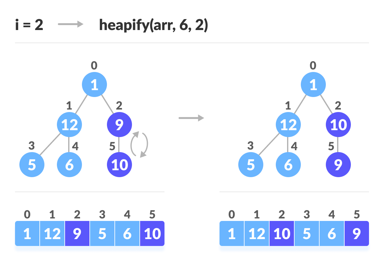
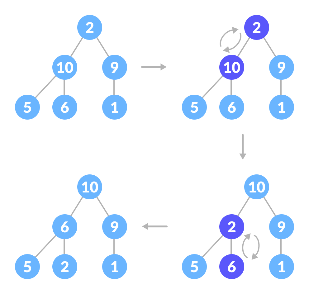
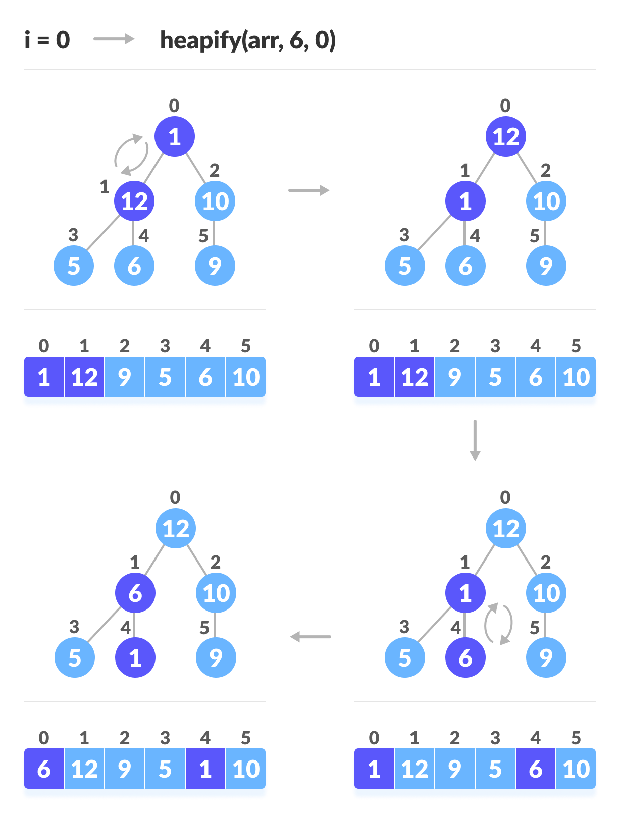
Selection Sort Algorithm
Selection sort is a sorting algorithm that selects the smallest element from an unsorted list in each iteration and places that element at the beginning of the unsorted list.
Working of Selection Sort
- Set the first element as
minimum.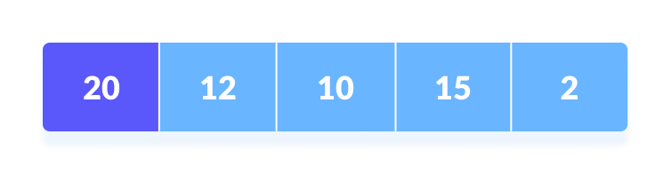
Select first element as minimum - Compare
minimumwith the second element. If the second element is smaller thanminimum, assign the second element asminimum.
Compareminimumwith the third element. Again, if the third element is smaller, then assignminimumto the third element otherwise do nothing. The process goes on until the last element.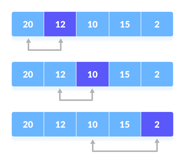
Compare minimum with the remaining elements - After each iteration,
minimumis placed in the front of the unsorted list.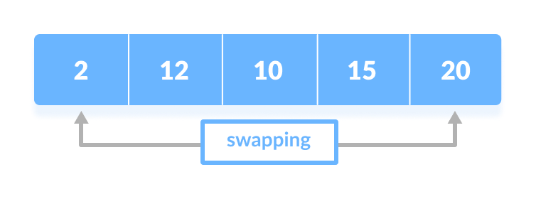
Swap the first with minimum - For each iteration, indexing starts from the first unsorted element. Step 1 to 3 are repeated until all the elements are placed at their correct positions.
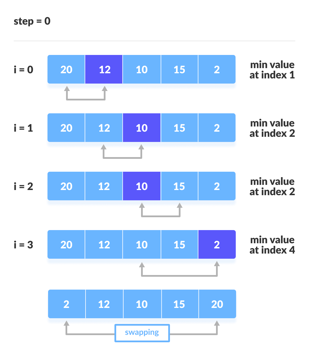
The first iteration 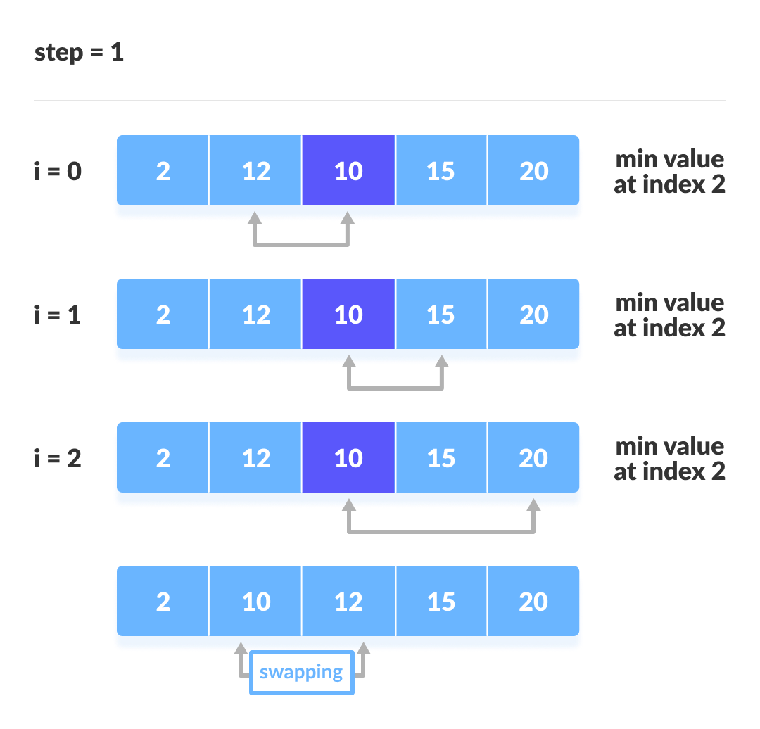
The second iteration 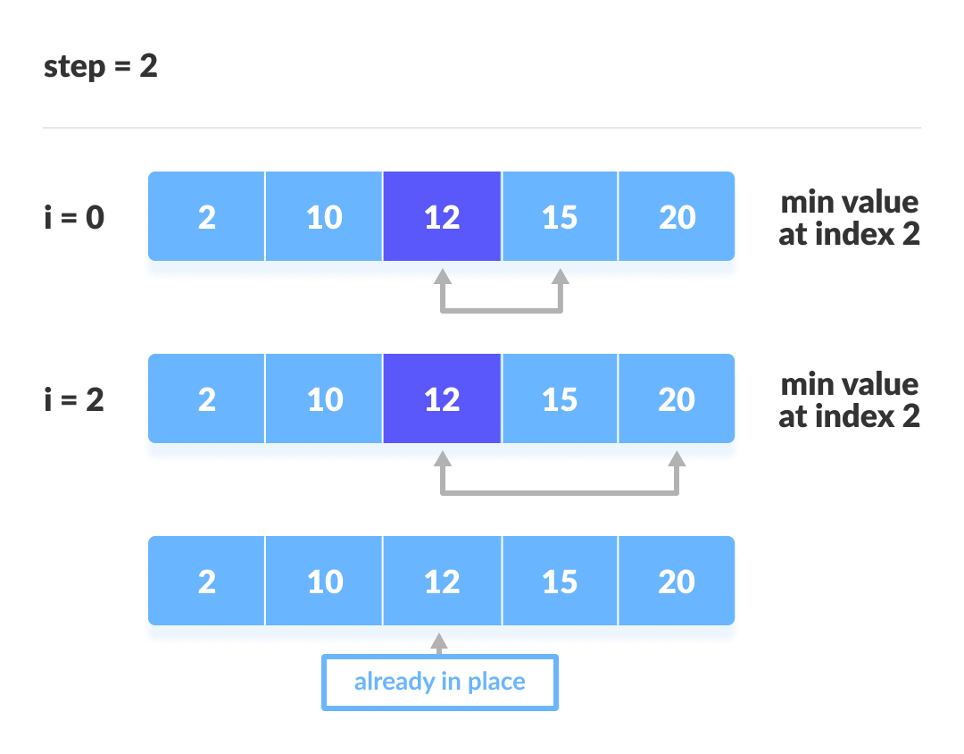
The third iteration 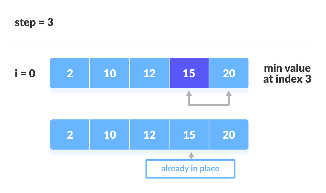
The fourth iteration
Selection Sort Algorithm
selectionSort(array, size)
  for i from 0 to size - 1 do
    set i as the index of the current minimum
    for j from i + 1 to size - 1 do
      if array[j] < array[current minimum]
        set j as the new current minimum index
    if current minimum is not i
      swap array[i] with array[current minimum]
end selectionSort
Selection Sort Code in Python, Java, and C/C++
# Selection sort in Python


def selectionSort(array, size):

    for step in range(size):
        min_idx = step

        for i in range(step + 1, size):

            # to sort in descending order, change > to < in this line
            # select the minimum element in each loop
            if array[i] < array[min_idx]:
                min_idx = i

        # put min at the correct position
        (array[step], array[min_idx]) = (array[min_idx], array[step])


data = [-2, 45, 0, 11, -9]
size = len(data)
selectionSort(data, size)
print('Sorted Array in Ascending Order:')
print(data)
// Selection sort in Java

import java.util.Arrays;

class SelectionSort {
  void selectionSort(int array[]) {
    int size = array.length;

    for (int step = 0; step < size - 1; step++) {
      int min_idx = step;

      for (int i = step + 1; i < size; i++) {

        // To sort in descending order, change > to < in this line.
        // Select the minimum element in each loop.
        if (array[i] < array[min_idx]) {
          min_idx = i;
        }
      }

      // put min at the correct position
      int temp = array[step];
      array[step] = array[min_idx];
      array[min_idx] = temp;
    }
  }

  // driver code
  public static void main(String args[]) {
    int[] data = { 20, 12, 10, 15, 2 };
    SelectionSort ss = new SelectionSort();
    ss.selectionSort(data);
    System.out.println("Sorted Array in Ascending Order: ");
    System.out.println(Arrays.toString(data));
  }
}
// Selection sort in C

#include <stdio.h>

// function to swap the the position of two elements
void swap(int *a, int *b) {
  int temp = *a;
  *a = *b;
  *b = temp;
}

void selectionSort(int array[], int size) {
  for (int step = 0; step < size - 1; step++) {
    int min_idx = step;
    for (int i = step + 1; i < size; i++) {

      // To sort in descending order, change > to < in this line.
      // Select the minimum element in each loop.
      if (array[i] < array[min_idx])
        min_idx = i;
    }

    // put min at the correct position
    swap(&array[min_idx], &array[step]);
  }
}

// function to print an array
void printArray(int array[], int size) {
  for (int i = 0; i < size; ++i) {
    printf("%d  ", array[i]);
  }
  printf("\n");
}

// driver code
int main() {
  int data[] = {20, 12, 10, 15, 2};
  int size = sizeof(data) / sizeof(data[0]);
  selectionSort(data, size);
  printf("Sorted array in Acsending Order:\n");
  printArray(data, size);
}
// Selection sort in C++

#include <iostream>
using namespace std;

// function to swap the the position of two elements
void swap(int *a, int *b) {
  int temp = *a;
  *a = *b;
  *b = temp;
}

// function to print an array
void printArray(int array[], int size) {
  for (int i = 0; i < size; i++) {
    cout << array[i] << " ";
  }
  cout << endl;
}

void selectionSort(int array[], int size) {
  for (int step = 0; step < size - 1; step++) {
    int min_idx = step;
    for (int i = step + 1; i < size; i++) {

      // To sort in descending order, change > to < in this line.
      // Select the minimum element in each loop.
      if (array[i] < array[min_idx])
        min_idx = i;
    }

    // put min at the correct position
    swap(&array[min_idx], &array[step]);
  }
}

// driver code
int main() {
  int data[] = {20, 12, 10, 15, 2};
  int size = sizeof(data) / sizeof(data[0]);
  selectionSort(data, size);
  cout << "Sorted array in Acsending Order:\n";
  printArray(data, size);
}
Selection Sort Complexity
| Time Complexity | |
|---|---|
| Best | O(n2) |
| Worst | O(n2) |
| Average | O(n2) |
| Space Complexity | O(1) |
| Stability | No |
| Cycle | Number of Comparison |
|---|---|
| 1st | (n-1) |
| 2nd | (n-2) |
| 3rd | (n-3) |
| ... | ... |
| last | 1 |
Number of comparisons: (n - 1) + (n - 2) + (n - 3) + ..... + 1 = n(n - 1) / 2 nearly equals to n2.
Complexity = O(n2)
Also, we can analyze the complexity by simply observing the number of loops. There are 2 loops so the complexity is n*n = n2.
Time Complexities:
- Worst Case Complexity:
O(n2)
If we want to sort in ascending order and the array is in descending order then, the worst case occurs. - Best Case Complexity:
O(n2)
It occurs when the array is already sorted - Average Case Complexity:
O(n2)
It occurs when the elements of the array are in jumbled order (neither ascending nor descending).
The time complexity of the selection sort is the same in all cases. At every step, you have to find the minimum element and put it in the right place. The minimum element is not known until the end of the array is not reached.
Space Complexity:
Space complexity is O(1) because an extra variable min_idx is used.
Selection Sort Applications
The selection sort is used when
- a small list is to be sorted
- cost of swapping does not matter
- checking of all the elements is compulsory
- cost of writing to a memory matters like in flash memory (number of writes/swaps is
O(n)as compared toO(n2)of bubble sort)
Similar Sorting Algorithms
Insertion Sort Algorithm
Insertion sort is a sorting algorithm that places an unsorted element at its suitable place in each iteration.
Insertion sort works similarly as we sort cards in our hand in a card game.
We assume that the first card is already sorted then, we select an unsorted card. If the unsorted card is greater than the card in hand, it is placed on the right otherwise, to the left. In the same way, other unsorted cards are taken and put in their right place.
A similar approach is used by insertion sort.
Working of Insertion Sort
Suppose we need to sort the following array.
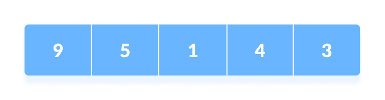
- The first element in the array is assumed to be sorted. Take the second element and store it separately in
key.
Comparekeywith the first element. If the first element is greater thankey, then key is placed in front of the first element.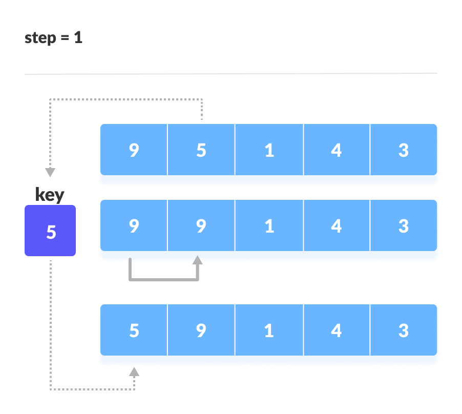
If the first element is greater than key, then key is placed in front of the first element. - Now, the first two elements are sorted.
Take the third element and compare it with the elements on the left of it. Placed it just behind the element smaller than it. If there is no element smaller than it, then place it at the beginning of the array.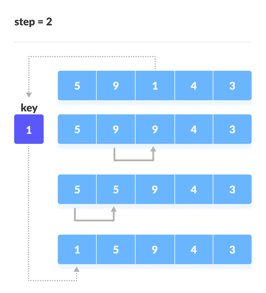
Place 1 at the beginning - Similarly, place every unsorted element at its correct position.
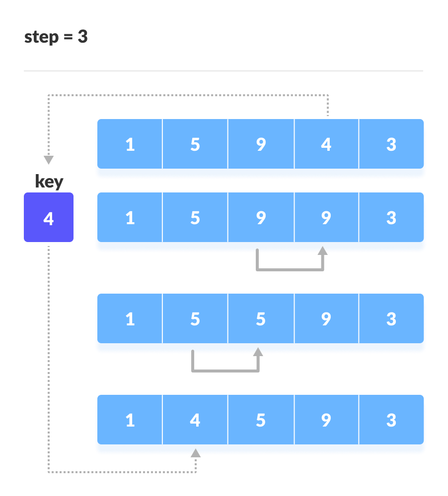
Place 4 behind 1 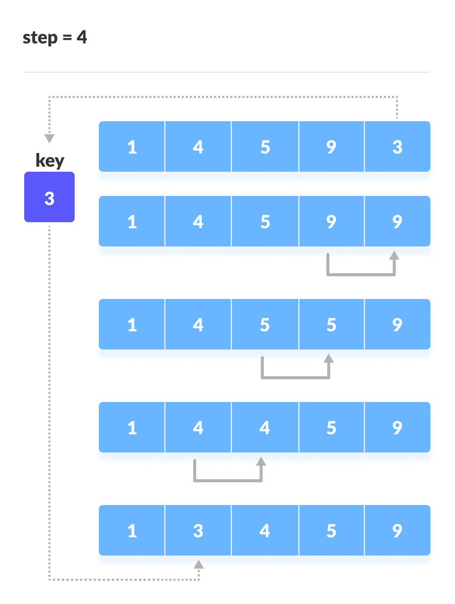
Place 3 behind 1 and the array is sorted
Insertion Sort Algorithm
insertionSort(array)
  mark first element as sorted
  for each unsorted element X
    'extract' the element X
    for j <- lastSortedIndex down to 0
      if current element j > X
        move sorted element to the right by 1
    break loop and insert X here
end insertionSort
Insertion Sort in Python, Java, and C/C++
# Insertion sort in Python


def insertionSort(array):

    for step in range(1, len(array)):
        key = array[step]
        j = step - 1

        # Compare key with each element on the left of it until an element smaller than it is found
        # For descending order, change key<array[j] to key>array[j].
        while j >= 0 and key < array[j]:
            array[j + 1] = array[j]
            j = j - 1

        # Place key at after the element just smaller than it.
        array[j + 1] = key


data = [9, 5, 1, 4, 3]
insertionSort(data)
print('Sorted Array in Ascending Order:')
print(data)
// Insertion sort in Java

import java.util.Arrays;

class InsertionSort {

  void insertionSort(int array[]) {
    int size = array.length;

    for (int step = 1; step < size; step++) {
      int key = array[step];
      int j = step - 1;

      // Compare key with each element on the left of it until an element smaller than
      // it is found.
      // For descending order, change key<array[j] to key>array[j].
      while (j >= 0 && key < array[j]) {
        array[j + 1] = array[j];
        --j;
      }

      // Place key at after the element just smaller than it.
      array[j + 1] = key;
    }
  }

  // Driver code
  public static void main(String args[]) {
    int[] data = { 9, 5, 1, 4, 3 };
    InsertionSort is = new InsertionSort();
    is.insertionSort(data);
    System.out.println("Sorted Array in Ascending Order: ");
    System.out.println(Arrays.toString(data));
  }
}
// Insertion sort in C

#include <stdio.h>

// Function to print an array
void printArray(int array[], int size) {
  for (int i = 0; i < size; i++) {
    printf("%d ", array[i]);
  }
  printf("\n");
}

void insertionSort(int array[], int size) {
  for (int step = 1; step < size; step++) {
    int key = array[step];
    int j = step - 1;

    // Compare key with each element on the left of it until an element smaller than
    // it is found.
    // For descending order, change key<array[j] to key>array[j].
    while (j >=0 && key < array[j]) {
      array[j + 1] = array[j];
      --j;
    }
    array[j + 1] = key;
  }
}

// Driver code
int main() {
  int data[] = {9, 5, 1, 4, 3};
  int size = sizeof(data) / sizeof(data[0]);
  insertionSort(data, size);
  printf("Sorted array in ascending order:\n");
  printArray(data, size);
}
// Insertion sort in C++

#include <iostream>
using namespace std;

// Function to print an array
void printArray(int array[], int size) {
  for (int i = 0; i < size; i++) {
    cout << array[i] << " ";
  }
  cout << endl;
}

void insertionSort(int array[], int size) {
  for (int step = 1; step < size; step++) {
    int key = array[step];
    int j = step - 1;

    // Compare key with each element on the left of it until an element smaller than
    // it is found.
    // For descending order, change key<array[j] to key>array[j].
    while (j >=0 && key < array[j]) {
      array[j + 1] = array[j];
      --j;
    }
    array[j + 1] = key;
  }
}

// Driver code
int main() {
  int data[] = {9, 5, 1, 4, 3};
  int size = sizeof(data) / sizeof(data[0]);
  insertionSort(data, size);
  cout << "Sorted array in ascending order:\n";
  printArray(data, size);
}
Insertion Sort Complexity
| Time Complexity | |
|---|---|
| Best | O(n) |
| Worst | O(n2) |
| Average | O(n2) |
| Space Complexity | O(1) |
| Stability | Yes |
Time Complexities
- Worst Case Complexity:
O(n2)
Suppose, an array is in ascending order, and you want to sort it in descending order. In this case, worst case complexity occurs.
Each element has to be compared with each of the other elements so, for every nth element,(n-1)number of comparisons are made.
Thus, the total number of comparisons =n*(n-1) ~ n2 - Best Case Complexity:
O(n)
When the array is already sorted, the outer loop runs fornnumber of times whereas the inner loop does not run at all. So, there are onlynnumber of comparisons. Thus, complexity is linear. - Average Case Complexity:
O(n2)
It occurs when the elements of an array are in jumbled order (neither ascending nor descending).
Space Complexity
Space complexity is O(1) because an extra variable key is used.
Insertion Sort Applications
The insertion sort is used when:
- the array is has a small number of elements
- there are only a few elements left to be sorted
Similar Sorting Algorithms