
Dynamic Programming
Dynamic Programming is a technique in computer programming that helps to efficiently solve a class of problems that have overlapping subproblems and optimal substructure property.
If any problem can be divided into subproblems, which in turn are divided into smaller subproblems, and if there are overlapping among these subproblems, then the solutions to these subproblems can be saved for future reference. In this way, efficiency of the CPU can be enhanced. This method of solving a solution is referred to as dynamic programming.
Such problems involve repeatedly calculating the value of the same subproblems to find the optimum solution.
Dynamic Programming Example
Let's find the fibonacci sequence upto 5th term. A fibonacci series is the sequence of numbers in which each number is the sum of the two preceding ones. For example, 0,1,1, 2, 3. Here, each number is the sum of the two preceding numbers.
Algorithm
Let n be the number of terms.

1. If n = 0, return 0.
2. If n = 1, return 1.
3. Else, return the sum of two preceding numbers.
We are calculating the fibonacci sequence up to the 5th term.
- The first term is 0.
- The second term is 1.
- The third term is sum of 0 (from step 1) and 1(from step 2), which is 1.
- The fourth term is the sum of the third term (from step 3) and second term (from step 2) i.e.
1 + 1 = 2. - The fifth term is the sum of the fourth term (from step 4) and third term (from step 3) i.e.
2 + 1 = 3.
Hence, we have the sequence 0,1,1, 2, 3. Here, we have used the results of the previous steps as shown below. This is called a dynamic programming approach.
F(0) = 0
F(1) = 1
F(2) = F(1) + F(0)
F(3) = F(2) + F(1)
F(4) = F(3) + F(2)
How Dynamic Programming Works
Dynamic programming works by storing the result of subproblems so that when their solutions are required, they are at hand and we do not need to recalculate them.
This technique of storing the value of subproblems is called memoization. By saving the values in the array, we save time for computations of sub-problems we have already come across.
var m = map(0 → 0, 1 → 1)
function fib(n)
    if key n is not in map m
        m[n] = fib(n − 1) + fib(n − 2)
    return m[n]
Dynamic programming by memoization is a top-down approach to dynamic programming. By reversing the direction in which the algorithm works i.e. by starting from the base case and working towards the solution, we can also implement dynamic programming in a bottom-up manner.
function fib(n)
    if n = 0
        return 0
    else
        var prevFib = 0, currFib = 1
        repeat n − 1 times
            var newFib = prevFib + currFib
            prevFib = currFib
            currFib  = newFib
    return currentFib
Recursion vs Dynamic Programming
Dynamic programming is mostly applied to recursive algorithms. This is not a coincidence, most optimization problems require recursion and dynamic programming is used for optimization.
But not all problems that use recursion can use Dynamic Programming. Unless there is a presence of overlapping subproblems like in the fibonacci sequence problem, a recursion can only reach the solution using a divide and conquer approach.
That is the reason why a recursive algorithm like Merge Sort cannot use Dynamic Programming, because the subproblems are not overlapping in any way.
Greedy Algorithms vs Dynamic Programming
Greedy Algorithms are similar to dynamic programming in the sense that they are both tools for optimization.
However, greedy algorithms look for locally optimum solutions or in other words, a greedy choice, in the hopes of finding a global optimum. Hence greedy algorithms can make a guess that looks optimum at the time but becomes costly down the line and do not guarantee a globally optimum.
Dynamic programming, on the other hand, finds the optimal solution to subproblems and then makes an informed choice to combine the results of those subproblems to find the most optimum solution.
Different Types of Dynamic Programming Algorithms
Prim's Algorithm
Prim's algorithm is a minimum spanning tree algorithm that takes a graph as input and finds the subset of the edges of that graph which
- form a tree that includes every vertex
- has the minimum sum of weights among all the trees that can be formed from the graph
How Prim's algorithm works
It falls under a class of algorithms called greedy algorithms that find the local optimum in the hopes of finding a global optimum.
We start from one vertex and keep adding edges with the lowest weight until we reach our goal.
The steps for implementing Prim's algorithm are as follows:
- Initialize the minimum spanning tree with a vertex chosen at random.
- Find all the edges that connect the tree to new vertices, find the minimum and add it to the tree
- Keep repeating step 2 until we get a minimum spanning tree
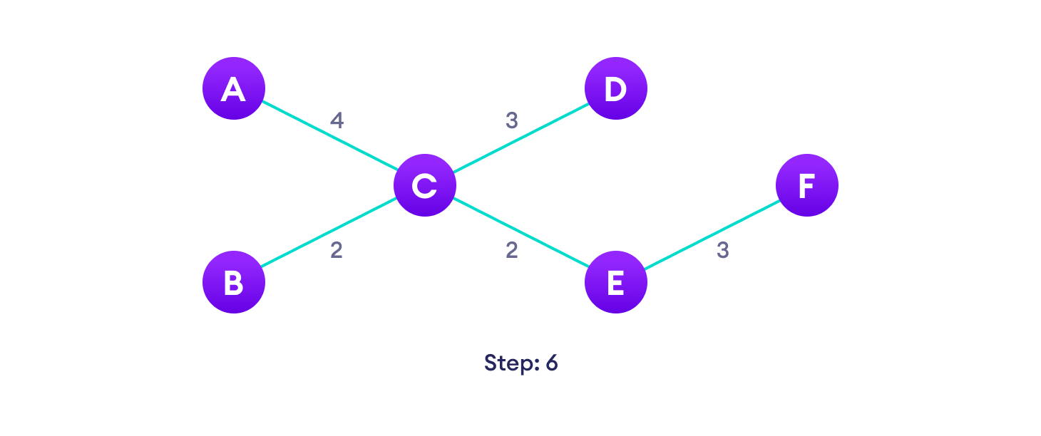
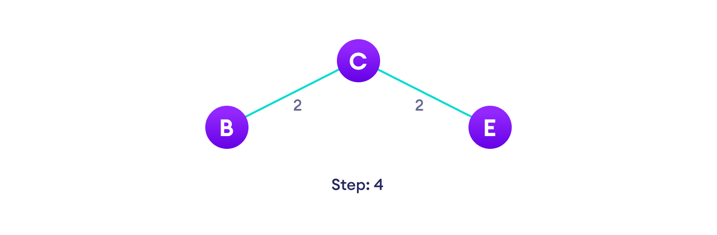
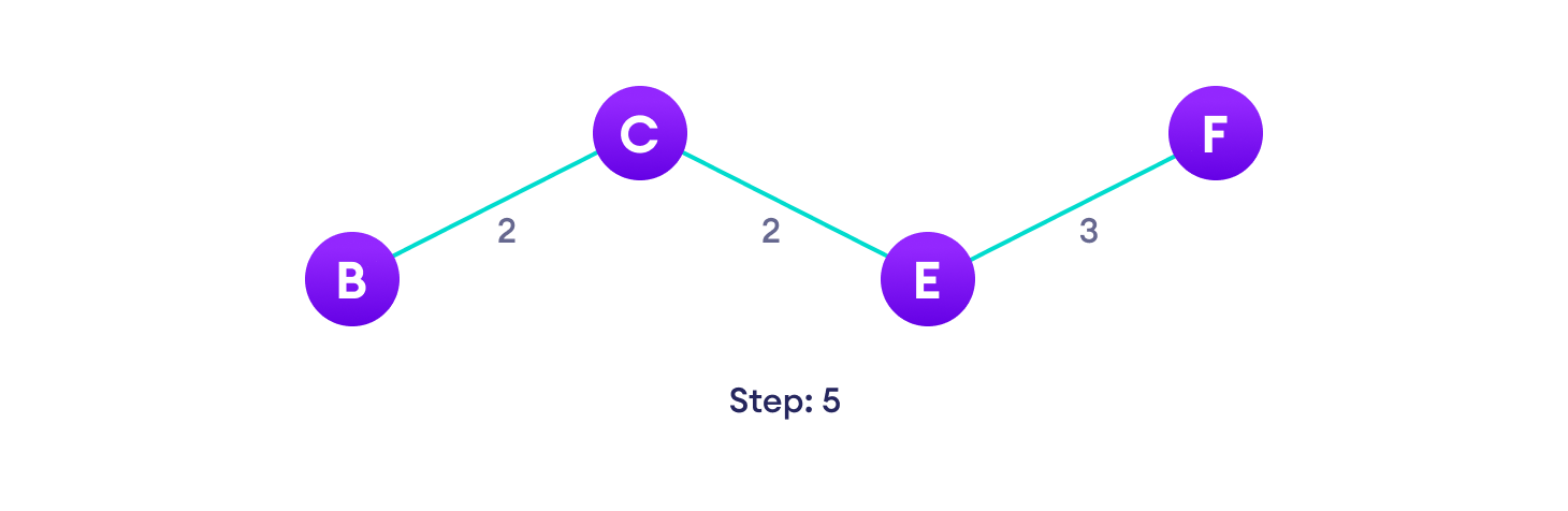
Example of Prim's algorithm
Prim's Algorithm pseudocode
The pseudocode for prim's algorithm shows how we create two sets of vertices U and V-U. U contains the list of vertices that have been visited and V-U the list of vertices that haven't. One by one, we move vertices from set V-U to set U by connecting the least weight edge.
T = ∅;
U = { 1 };
while (U ≠ V)
    let (u, v) be the lowest cost edge such that u ∈ U and v ∈ V - U;
    T = T ∪ {(u, v)}
    U = U ∪ {v}
Python, Java and C/C++ Examples
Although adjacency matrix representation of graphs is used, this algorithm can also be implemented using Adjacency List to improve its efficiency.
# Prim's Algorithm in Python


INF = 9999999
# number of vertices in graph
V = 5
# create a 2d array of size 5x5
# for adjacency matrix to represent graph
G = [[0, 9, 75, 0, 0],
     [9, 0, 95, 19, 42],
     [75, 95, 0, 51, 66],
     [0, 19, 51, 0, 31],
     [0, 42, 66, 31, 0]]
# create a array to track selected vertex
# selected will become true otherwise false
selected = [0, 0, 0, 0, 0]
# set number of edge to 0
no_edge = 0
# the number of egde in minimum spanning tree will be
# always less than(V - 1), where V is number of vertices in
# graph
# choose 0th vertex and make it true
selected[0] = True
# print for edge and weight
print("Edge : Weight\n")
while (no_edge < V - 1):
    # For every vertex in the set S, find the all adjacent vertices
    #, calculate the distance from the vertex selected at step 1.
    # if the vertex is already in the set S, discard it otherwise
    # choose another vertex nearest to selected vertex  at step 1.
    minimum = INF
    x = 0
    y = 0
    for i in range(V):
        if selected[i]:
            for j in range(V):
                if ((not selected[j]) and G[i][j]):
                    # not in selected and there is an edge
                    if minimum > G[i][j]:
                        minimum = G[i][j]
                        x = i
                        y = j
    print(str(x) + "-" + str(y) + ":" + str(G[x][y]))
    selected[y] = True
    no_edge += 1
// Prim's Algorithm in Java

import java.util.Arrays;

class PGraph {

  public void Prim(int G[][], int V) {

    int INF = 9999999;

    int no_edge; // number of edge

    // create a array to track selected vertex
    // selected will become true otherwise false
    boolean[] selected = new boolean[V];

    // set selected false initially
    Arrays.fill(selected, false);

    // set number of edge to 0
    no_edge = 0;

    // the number of egde in minimum spanning tree will be
    // always less than (V -1), where V is number of vertices in
    // graph

    // choose 0th vertex and make it true
    selected[0] = true;

    // print for edge and weight
    System.out.println("Edge : Weight");

    while (no_edge < V - 1) {
      // For every vertex in the set S, find the all adjacent vertices
      // , calculate the distance from the vertex selected at step 1.
      // if the vertex is already in the set S, discard it otherwise
      // choose another vertex nearest to selected vertex at step 1.

      int min = INF;
      int x = 0; // row number
      int y = 0; // col number

      for (int i = 0; i < V; i++) {
        if (selected[i] == true) {
          for (int j = 0; j < V; j++) {
            // not in selected and there is an edge
            if (!selected[j] && G[i][j] != 0) {
              if (min > G[i][j]) {
                min = G[i][j];
                x = i;
                y = j;
              }
            }
          }
        }
      }
      System.out.println(x + " - " + y + " :  " + G[x][y]);
      selected[y] = true;
      no_edge++;
    }
  }

  public static void main(String[] args) {
    PGraph g = new PGraph();

    // number of vertices in grapj
    int V = 5;

    // create a 2d array of size 5x5
    // for adjacency matrix to represent graph
    int[][] G = { { 0, 9, 75, 0, 0 }, { 9, 0, 95, 19, 42 }, { 75, 95, 0, 51, 66 }, { 0, 19, 51, 0, 31 },
        { 0, 42, 66, 31, 0 } };

    g.Prim(G, V);
  }
}
// Prim's Algorithm in C

#include<stdio.h>
#include<stdbool.h>

#define INF 9999999

// number of vertices in graph
#define V 5

// create a 2d array of size 5x5
//for adjacency matrix to represent graph
int G[V][V] = {
  {0, 9, 75, 0, 0},
  {9, 0, 95, 19, 42},
  {75, 95, 0, 51, 66},
  {0, 19, 51, 0, 31},
  {0, 42, 66, 31, 0}};

int main() {
  int no_edge;  // number of edge

  // create a array to track selected vertex
  // selected will become true otherwise false
  int selected[V];

  // set selected false initially
  memset(selected, false, sizeof(selected));

  // set number of edge to 0
  no_edge = 0;

  // the number of egde in minimum spanning tree will be
  // always less than (V -1), where V is number of vertices in
  //graph

  // choose 0th vertex and make it true
  selected[0] = true;

  int x;  //  row number
  int y;  //  col number

  // print for edge and weight
  printf("Edge : Weight\n");

  while (no_edge < V - 1) {
    //For every vertex in the set S, find the all adjacent vertices
    // , calculate the distance from the vertex selected at step 1.
    // if the vertex is already in the set S, discard it otherwise
    //choose another vertex nearest to selected vertex  at step 1.

    int min = INF;
    x = 0;
    y = 0;

    for (int i = 0; i < V; i++) {
      if (selected[i]) {
        for (int j = 0; j < V; j++) {
          if (!selected[j] && G[i][j]) {  // not in selected and there is an edge
            if (min > G[i][j]) {
              min = G[i][j];
              x = i;
              y = j;
            }
          }
        }
      }
    }
    printf("%d - %d : %d\n", x, y, G[x][y]);
    selected[y] = true;
    no_edge++;
  }

  return 0;
}
// Prim's Algorithm in C++

#include <cstring>
#include <iostream>
using namespace std;

#define INF 9999999

// number of vertices in grapj
#define V 5

// create a 2d array of size 5x5
//for adjacency matrix to represent graph

int G[V][V] = {
  {0, 9, 75, 0, 0},
  {9, 0, 95, 19, 42},
  {75, 95, 0, 51, 66},
  {0, 19, 51, 0, 31},
  {0, 42, 66, 31, 0}};

int main() {
  int no_edge;  // number of edge

  // create a array to track selected vertex
  // selected will become true otherwise false
  int selected[V];

  // set selected false initially
  memset(selected, false, sizeof(selected));

  // set number of edge to 0
  no_edge = 0;

  // the number of egde in minimum spanning tree will be
  // always less than (V -1), where V is number of vertices in
  //graph

  // choose 0th vertex and make it true
  selected[0] = true;

  int x;  //  row number
  int y;  //  col number

  // print for edge and weight
  cout << "Edge"
     << " : "
     << "Weight";
  cout << endl;
  while (no_edge < V - 1) {
    //For every vertex in the set S, find the all adjacent vertices
    // , calculate the distance from the vertex selected at step 1.
    // if the vertex is already in the set S, discard it otherwise
    //choose another vertex nearest to selected vertex  at step 1.

    int min = INF;
    x = 0;
    y = 0;

    for (int i = 0; i < V; i++) {
      if (selected[i]) {
        for (int j = 0; j < V; j++) {
          if (!selected[j] && G[i][j]) {  // not in selected and there is an edge
            if (min > G[i][j]) {
              min = G[i][j];
              x = i;
              y = j;
            }
          }
        }
      }
    }
    cout << x << " - " << y << " :  " << G[x][y];
    cout << endl;
    selected[y] = true;
    no_edge++;
  }

  return 0;
}
Prim's vs Kruskal's Algorithm
Kruskal's algorithm is another popular minimum spanning tree algorithm that uses a different logic to find the MST of a graph. Instead of starting from a vertex, Kruskal's algorithm sorts all the edges from low weight to high and keeps adding the lowest edges, ignoring those edges that create a cycle.
Prim's Algorithm Complexity
The time complexity of Prim's algorithm is O(V2).
Prim's Algorithm Application
- Laying cables of electrical wiring
- In network designed
- To make protocols in network cycles
Kruskal's Algorithm
Kruskal's algorithm is a minimum spanning tree algorithm that takes a graph as input and finds the subset of the edges of that graph which
- form a tree that includes every vertex
- has the minimum sum of weights among all the trees that can be formed from the graph
How Kruskal's algorithm works
It falls under a class of algorithms called greedy algorithms that find the local optimum in the hopes of finding a global optimum.
We start from the edges with the lowest weight and keep adding edges until we reach our goal.
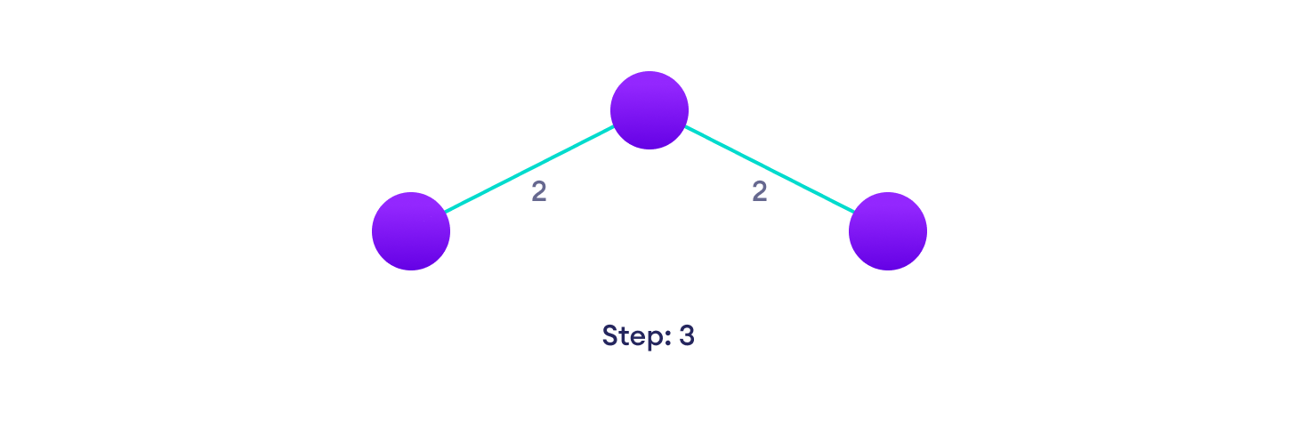
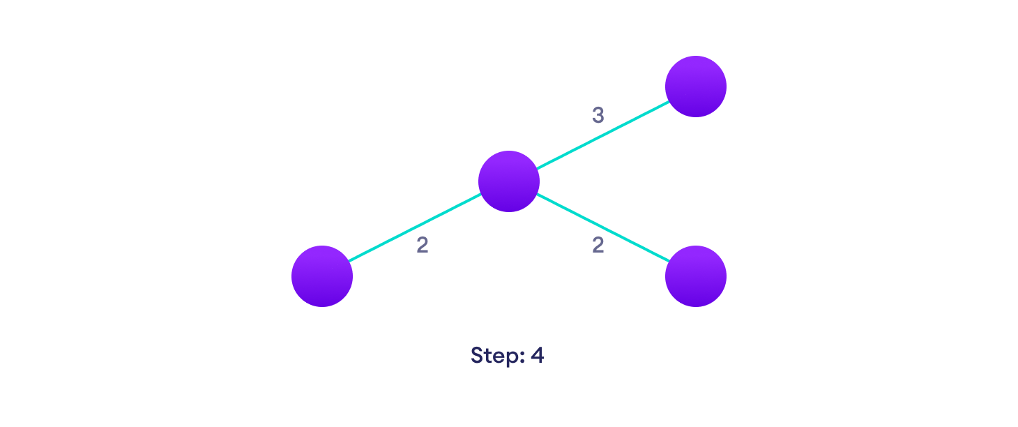
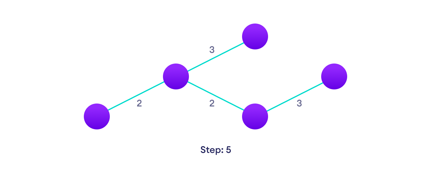
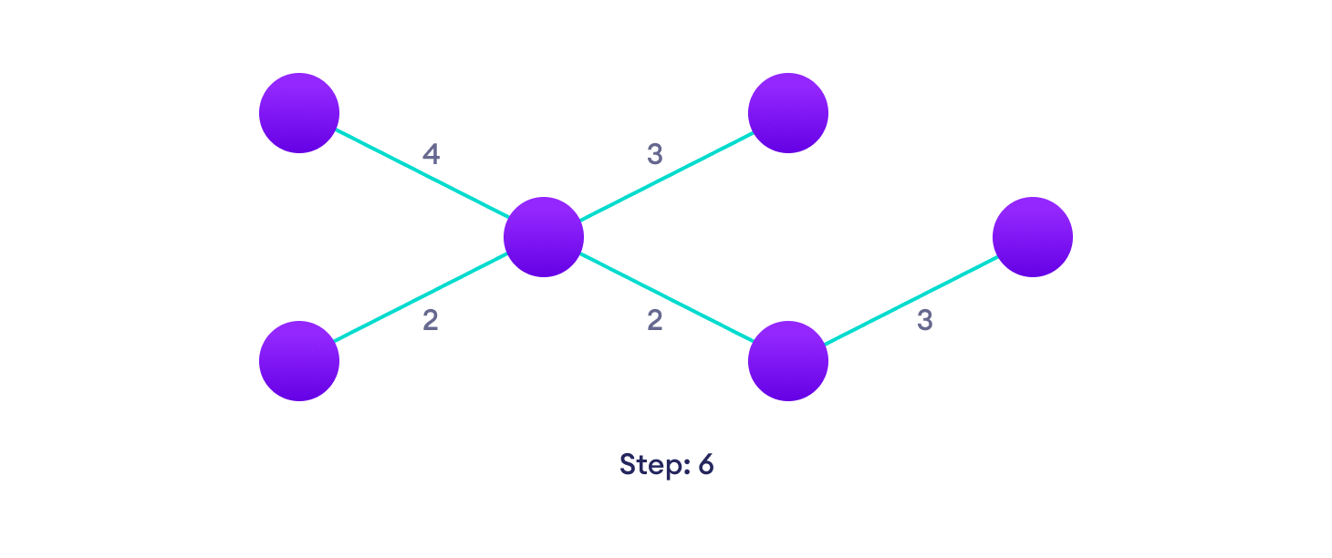
The steps for implementing Kruskal's algorithm are as follows:
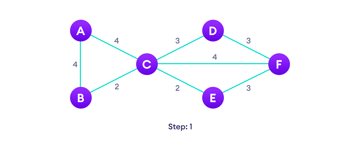
- Sort all the edges from low weight to high
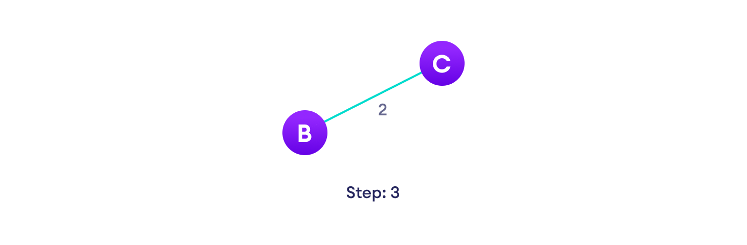
- Take the edge with the lowest weight and add it to the spanning tree. If adding the edge created a cycle, then reject this edge.
- Keep adding edges until we reach all vertices.
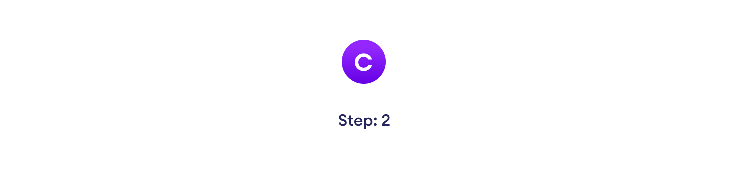
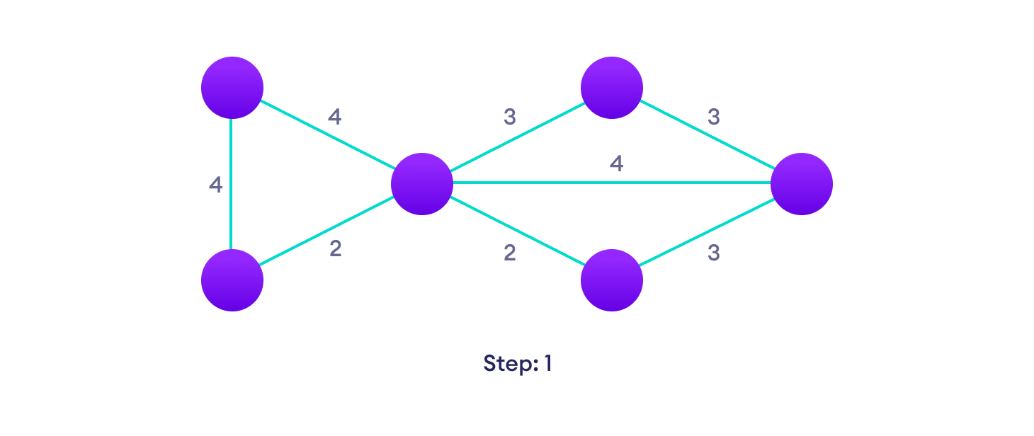
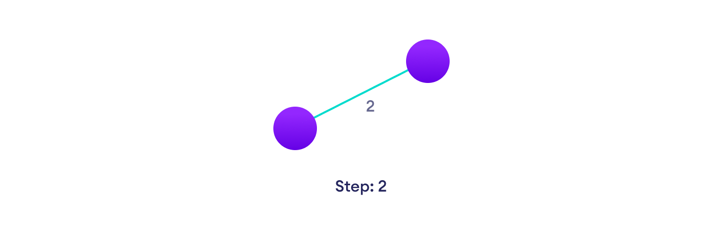
Example of Kruskal's algorithm
Kruskal Algorithm Pseudocode
Any minimum spanning tree algorithm revolves around checking if adding an edge creates a loop or not.
The most common way to find this out is an algorithm called Union FInd. The Union-Find algorithm divides the vertices into clusters and allows us to check if two vertices belong to the same cluster or not and hence decide whether adding an edge creates a cycle.
KRUSKAL(G):
A = ∅
For each vertex v ∈ G.V:
    MAKE-SET(v)
For each edge (u, v) ∈ G.E ordered by increasing order by weight(u, v):
    if FIND-SET(u) ≠ FIND-SET(v):
    A = A ∪ {(u, v)}
    UNION(u, v)
return A
Python, Java and C/C++ Examples
# Kruskal's algorithm in Python


class Graph:
    def __init__(self, vertices):
        self.V = vertices
        self.graph = []

    def add_edge(self, u, v, w):
        self.graph.append([u, v, w])

    # Search function

    def find(self, parent, i):
        if parent[i] == i:
            return i
        return self.find(parent, parent[i])

    def apply_union(self, parent, rank, x, y):
        xroot = self.find(parent, x)
        yroot = self.find(parent, y)
        if rank[xroot] < rank[yroot]:
            parent[xroot] = yroot
        elif rank[xroot] > rank[yroot]:
            parent[yroot] = xroot
        else:
            parent[yroot] = xroot
            rank[xroot] += 1

    #  Applying Kruskal algorithm
    def kruskal_algo(self):
        result = []
        i, e = 0, 0
        self.graph = sorted(self.graph, key=lambda item: item[2])
        parent = []
        rank = []
        for node in range(self.V):
            parent.append(node)
            rank.append(0)
        while e < self.V - 1:
            u, v, w = self.graph[i]
            i = i + 1
            x = self.find(parent, u)
            y = self.find(parent, v)
            if x != y:
                e = e + 1
                result.append([u, v, w])
                self.apply_union(parent, rank, x, y)
        for u, v, weight in result:
            print("%d - %d: %d" % (u, v, weight))


g = Graph(6)
g.add_edge(0, 1, 4)
g.add_edge(0, 2, 4)
g.add_edge(1, 2, 2)
g.add_edge(1, 0, 4)
g.add_edge(2, 0, 4)
g.add_edge(2, 1, 2)
g.add_edge(2, 3, 3)
g.add_edge(2, 5, 2)
g.add_edge(2, 4, 4)
g.add_edge(3, 2, 3)
g.add_edge(3, 4, 3)
g.add_edge(4, 2, 4)
g.add_edge(4, 3, 3)
g.add_edge(5, 2, 2)
g.add_edge(5, 4, 3)
g.kruskal_algo()
// Kruskal's algorithm in Java

import java.util.*;

class Graph {
  class Edge implements Comparable<Edge> {
    int src, dest, weight;

    public int compareTo(Edge compareEdge) {
      return this.weight - compareEdge.weight;
    }
  };

  // Union
  class subset {
    int parent, rank;
  };

  int vertices, edges;
  Edge edge[];

  // Graph creation
  Graph(int v, int e) {
    vertices = v;
    edges = e;
    edge = new Edge[edges];
    for (int i = 0; i < e; ++i)
      edge[i] = new Edge();
  }

  int find(subset subsets[], int i) {
    if (subsets[i].parent != i)
      subsets[i].parent = find(subsets, subsets[i].parent);
    return subsets[i].parent;
  }

  void Union(subset subsets[], int x, int y) {
    int xroot = find(subsets, x);
    int yroot = find(subsets, y);

    if (subsets[xroot].rank < subsets[yroot].rank)
      subsets[xroot].parent = yroot;
    else if (subsets[xroot].rank > subsets[yroot].rank)
      subsets[yroot].parent = xroot;
    else {
      subsets[yroot].parent = xroot;
      subsets[xroot].rank++;
    }
  }

  // Applying Krushkal Algorithm
  void KruskalAlgo() {
    Edge result[] = new Edge[vertices];
    int e = 0;
    int i = 0;
    for (i = 0; i < vertices; ++i)
      result[i] = new Edge();

    // Sorting the edges
    Arrays.sort(edge);
    subset subsets[] = new subset[vertices];
    for (i = 0; i < vertices; ++i)
      subsets[i] = new subset();

    for (int v = 0; v < vertices; ++v) {
      subsets[v].parent = v;
      subsets[v].rank = 0;
    }
    i = 0;
    while (e < vertices - 1) {
      Edge next_edge = new Edge();
      next_edge = edge[i++];
      int x = find(subsets, next_edge.src);
      int y = find(subsets, next_edge.dest);
      if (x != y) {
        result[e++] = next_edge;
        Union(subsets, x, y);
      }
    }
    for (i = 0; i < e; ++i)
      System.out.println(result[i].src + " - " + result[i].dest + ": " + result[i].weight);
  }

  public static void main(String[] args) {
    int vertices = 6; // Number of vertices
    int edges = 8; // Number of edges
    Graph G = new Graph(vertices, edges);

    G.edge[0].src = 0;
    G.edge[0].dest = 1;
    G.edge[0].weight = 4;

    G.edge[1].src = 0;
    G.edge[1].dest = 2;
    G.edge[1].weight = 4;

    G.edge[2].src = 1;
    G.edge[2].dest = 2;
    G.edge[2].weight = 2;

    G.edge[3].src = 2;
    G.edge[3].dest = 3;
    G.edge[3].weight = 3;

    G.edge[4].src = 2;
    G.edge[4].dest = 5;
    G.edge[4].weight = 2;

    G.edge[5].src = 2;
    G.edge[5].dest = 4;
    G.edge[5].weight = 4;

    G.edge[6].src = 3;
    G.edge[6].dest = 4;
    G.edge[6].weight = 3;

    G.edge[7].src = 5;
    G.edge[7].dest = 4;
    G.edge[7].weight = 3;
    G.KruskalAlgo();
  }
}
// Kruskal's algorithm in C

#include <stdio.h>

#define MAX 30

typedef struct edge {
  int u, v, w;
} edge;

typedef struct edge_list {
  edge data[MAX];
  int n;
} edge_list;

edge_list elist;

int Graph[MAX][MAX], n;
edge_list spanlist;

void kruskalAlgo();
int find(int belongs[], int vertexno);
void applyUnion(int belongs[], int c1, int c2);
void sort();
void print();

// Applying Krushkal Algo
void kruskalAlgo() {
  int belongs[MAX], i, j, cno1, cno2;
  elist.n = 0;

  for (i = 1; i < n; i++)
    for (j = 0; j < i; j++) {
      if (Graph[i][j] != 0) {
        elist.data[elist.n].u = i;
        elist.data[elist.n].v = j;
        elist.data[elist.n].w = Graph[i][j];
        elist.n++;
      }
    }

  sort();

  for (i = 0; i < n; i++)
    belongs[i] = i;

  spanlist.n = 0;

  for (i = 0; i < elist.n; i++) {
    cno1 = find(belongs, elist.data[i].u);
    cno2 = find(belongs, elist.data[i].v);

    if (cno1 != cno2) {
      spanlist.data[spanlist.n] = elist.data[i];
      spanlist.n = spanlist.n + 1;
      applyUnion(belongs, cno1, cno2);
    }
  }
}

int find(int belongs[], int vertexno) {
  return (belongs[vertexno]);
}

void applyUnion(int belongs[], int c1, int c2) {
  int i;

  for (i = 0; i < n; i++)
    if (belongs[i] == c2)
      belongs[i] = c1;
}

// Sorting algo
void sort() {
  int i, j;
  edge temp;

  for (i = 1; i < elist.n; i++)
    for (j = 0; j < elist.n - 1; j++)
      if (elist.data[j].w > elist.data[j + 1].w) {
        temp = elist.data[j];
        elist.data[j] = elist.data[j + 1];
        elist.data[j + 1] = temp;
      }
}

// Printing the result
void print() {
  int i, cost = 0;

  for (i = 0; i < spanlist.n; i++) {
    printf("\n%d - %d : %d", spanlist.data[i].u, spanlist.data[i].v, spanlist.data[i].w);
    cost = cost + spanlist.data[i].w;
  }

  printf("\nSpanning tree cost: %d", cost);
}

int main() {
  int i, j, total_cost;

  n = 6;

  Graph[0][0] = 0;
  Graph[0][1] = 4;
  Graph[0][2] = 4;
  Graph[0][3] = 0;
  Graph[0][4] = 0;
  Graph[0][5] = 0;
  Graph[0][6] = 0;

  Graph[1][0] = 4;
  Graph[1][1] = 0;
  Graph[1][2] = 2;
  Graph[1][3] = 0;
  Graph[1][4] = 0;
  Graph[1][5] = 0;
  Graph[1][6] = 0;

  Graph[2][0] = 4;
  Graph[2][1] = 2;
  Graph[2][2] = 0;
  Graph[2][3] = 3;
  Graph[2][4] = 4;
  Graph[2][5] = 0;
  Graph[2][6] = 0;

  Graph[3][0] = 0;
  Graph[3][1] = 0;
  Graph[3][2] = 3;
  Graph[3][3] = 0;
  Graph[3][4] = 3;
  Graph[3][5] = 0;
  Graph[3][6] = 0;

  Graph[4][0] = 0;
  Graph[4][1] = 0;
  Graph[4][2] = 4;
  Graph[4][3] = 3;
  Graph[4][4] = 0;
  Graph[4][5] = 0;
  Graph[4][6] = 0;

  Graph[5][0] = 0;
  Graph[5][1] = 0;
  Graph[5][2] = 2;
  Graph[5][3] = 0;
  Graph[5][4] = 3;
  Graph[5][5] = 0;
  Graph[5][6] = 0;

  kruskalAlgo();
  print();
}
// Kruskal's algorithm in C++

#include <algorithm>
#include <iostream>
#include <vector>
using namespace std;

#define edge pair<int, int>

class Graph {
   private:
  vector<pair<int, edge> > G;  // graph
  vector<pair<int, edge> > T;  // mst
  int *parent;
  int V;  // number of vertices/nodes in graph
   public:
  Graph(int V);
  void AddWeightedEdge(int u, int v, int w);
  int find_set(int i);
  void union_set(int u, int v);
  void kruskal();
  void print();
};
Graph::Graph(int V) {
  parent = new int[V];

  //i 0 1 2 3 4 5
  //parent[i] 0 1 2 3 4 5
  for (int i = 0; i < V; i++)
    parent[i] = i;

  G.clear();
  T.clear();
}
void Graph::AddWeightedEdge(int u, int v, int w) {
  G.push_back(make_pair(w, edge(u, v)));
}
int Graph::find_set(int i) {
  // If i is the parent of itself
  if (i == parent[i])
    return i;
  else
    // Else if i is not the parent of itself
    // Then i is not the representative of his set,
    // so we recursively call Find on its parent
    return find_set(parent[i]);
}

void Graph::union_set(int u, int v) {
  parent[u] = parent[v];
}
void Graph::kruskal() {
  int i, uRep, vRep;
  sort(G.begin(), G.end());  // increasing weight
  for (i = 0; i < G.size(); i++) {
    uRep = find_set(G[i].second.first);
    vRep = find_set(G[i].second.second);
    if (uRep != vRep) {
      T.push_back(G[i]);  // add to tree
      union_set(uRep, vRep);
    }
  }
}
void Graph::print() {
  cout << "Edge :"
     << " Weight" << endl;
  for (int i = 0; i < T.size(); i++) {
    cout << T[i].second.first << " - " << T[i].second.second << " : "
       << T[i].first;
    cout << endl;
  }
}
int main() {
  Graph g(6);
  g.AddWeightedEdge(0, 1, 4);
  g.AddWeightedEdge(0, 2, 4);
  g.AddWeightedEdge(1, 2, 2);
  g.AddWeightedEdge(1, 0, 4);
  g.AddWeightedEdge(2, 0, 4);
  g.AddWeightedEdge(2, 1, 2);
  g.AddWeightedEdge(2, 3, 3);
  g.AddWeightedEdge(2, 5, 2);
  g.AddWeightedEdge(2, 4, 4);
  g.AddWeightedEdge(3, 2, 3);
  g.AddWeightedEdge(3, 4, 3);
  g.AddWeightedEdge(4, 2, 4);
  g.AddWeightedEdge(4, 3, 3);
  g.AddWeightedEdge(5, 2, 2);
  g.AddWeightedEdge(5, 4, 3);
  g.kruskal();
  g.print();
  return 0;
}
Kruskal's vs Prim's Algorithm
Prim's algorithm is another popular minimum spanning tree algorithm that uses a different logic to find the MST of a graph. Instead of starting from an edge, Prim's algorithm starts from a vertex and keeps adding lowest-weight edges which aren't in the tree, until all vertices have been covered.
Kruskal's Algorithm Complexity
The time complexity Of Kruskal's Algorithm is: O(E log E).
Kruskal's Algorithm Applications
- In order to layout electrical wiring
- In computer network (LAN connection)
Breadth first search
Traversal means visiting all the nodes of a graph. Breadth First Traversal or Breadth First Search is a recursive algorithm for searching all the vertices of a graph or tree data structure.
BFS algorithm
A standard BFS implementation puts each vertex of the graph into one of two categories:
- Visited
- Not Visited
The purpose of the algorithm is to mark each vertex as visited while avoiding cycles.
The algorithm works as follows:
- Start by putting any one of the graph's vertices at the back of a queue.
- Take the front item of the queue and add it to the visited list.
- Create a list of that vertex's adjacent nodes. Add the ones which aren't in the visited list to the back of the queue.
- Keep repeating steps 2 and 3 until the queue is empty.
The graph might have two different disconnected parts so to make sure that we cover every vertex, we can also run the BFS algorithm on every node
BFS example
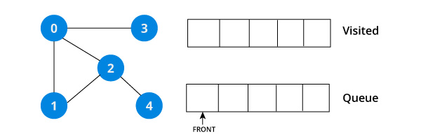
Let's see how the Breadth First Search algorithm works with an example. We use an undirected graph with 5 vertices.
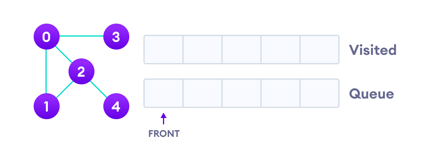
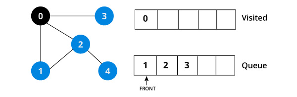
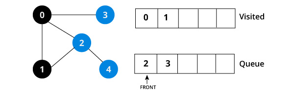
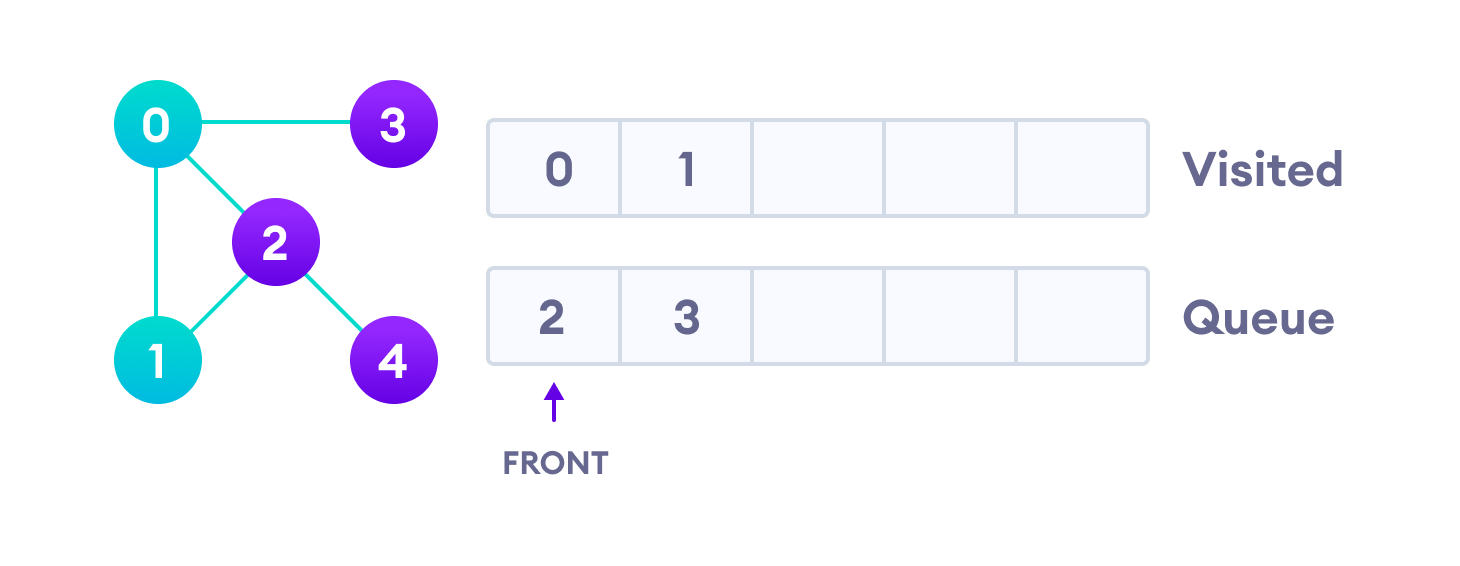
We start from vertex 0, the BFS algorithm starts by putting it in the Visited list and putting all its adjacent vertices in the queue.
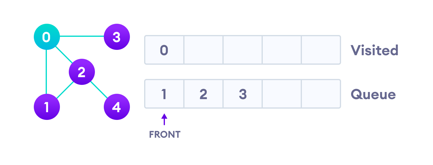
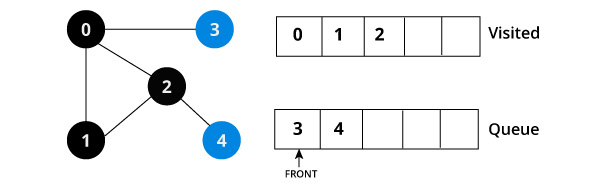
Next, we visit the element at the front of queue i.e. 1 and go to its adjacent nodes. Since 0 has already been visited, we visit 2 instead.
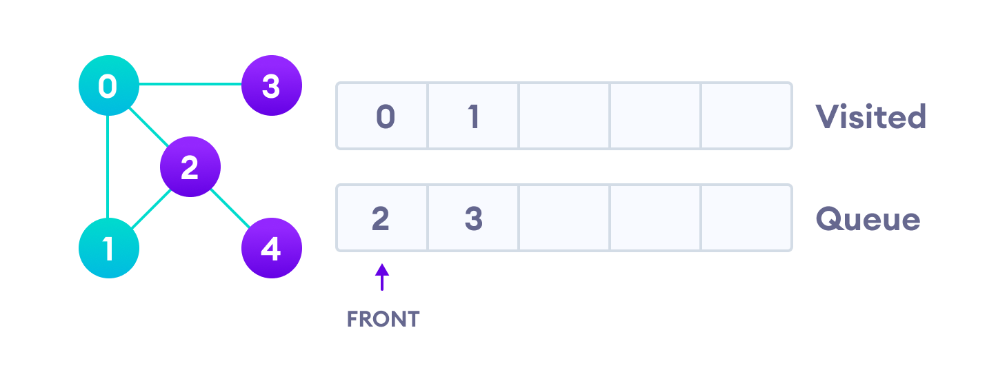
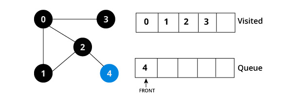
Vertex 2 has an unvisited adjacent vertex in 4, so we add that to the back of the queue and visit 3, which is at the front of the queue.
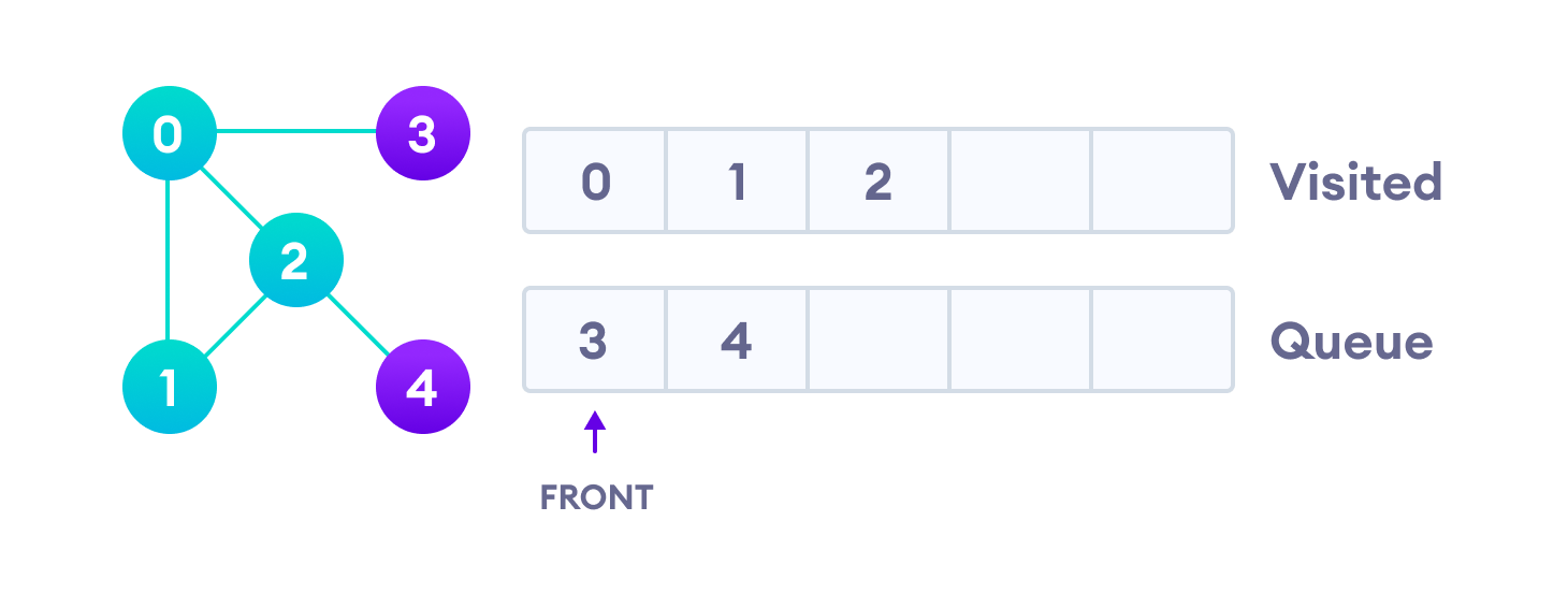
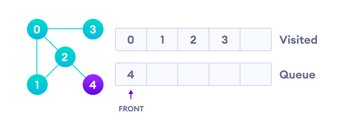
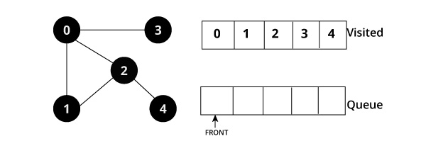
Only 4 remains in the queue since the only adjacent node of 3 i.e. 0 is already visited. We visit it.
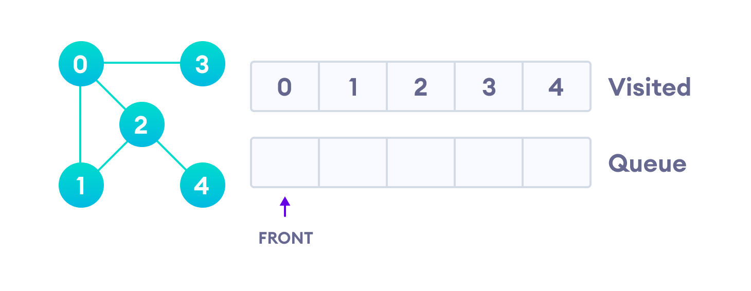
Since the queue is empty, we have completed the Breadth First Traversal of the graph.
BFS pseudocode
create a queue Q
mark v as visited and put v into Q
while Q is non-empty
    remove the head u of Q
    mark and enqueue all (unvisited) neighbours of u
Python, Java and C/C++ Examples
The code for the Breadth First Search Algorithm with an example is shown below. The code has been simplified so that we can focus on the algorithm rather than other details.
# BFS algorithm in Python


import collections

# BFS algorithm
def bfs(graph, root):

    visited, queue = set(), collections.deque([root])
    visited.add(root)

    while queue:

        # Dequeue a vertex from queue
        vertex = queue.popleft()
        print(str(vertex) + " ", end="")

        # If not visited, mark it as visited, and
        # enqueue it
        for neighbour in graph[vertex]:
            if neighbour not in visited:
                visited.add(neighbour)
                queue.append(neighbour)


if __name__ == '__main__':
    graph = {0: [1, 2], 1: [2], 2: [3], 3: [1, 2]}
    print("Following is Breadth First Traversal: ")
    bfs(graph, 0)
// BFS algorithm in Java

import java.util.*;

public class Graph {
  private int V;
  private LinkedList<Integer> adj[];

  // Create a graph
  Graph(int v) {
    V = v;
    adj = new LinkedList[v];
    for (int i = 0; i < v; ++i)
      adj[i] = new LinkedList();
  }

  // Add edges to the graph
  void addEdge(int v, int w) {
    adj[v].add(w);
  }

  // BFS algorithm
  void BFS(int s) {

    boolean visited[] = new boolean[V];

    LinkedList<Integer> queue = new LinkedList();

    visited[s] = true;
    queue.add(s);

    while (queue.size() != 0) {
      s = queue.poll();
      System.out.print(s + " ");

      Iterator<Integer> i = adj[s].listIterator();
      while (i.hasNext()) {
        int n = i.next();
        if (!visited[n]) {
          visited[n] = true;
          queue.add(n);
        }
      }
    }
  }

  public static void main(String args[]) {
    Graph g = new Graph(4);

    g.addEdge(0, 1);
    g.addEdge(0, 2);
    g.addEdge(1, 2);
    g.addEdge(2, 0);
    g.addEdge(2, 3);
    g.addEdge(3, 3);

    System.out.println("Following is Breadth First Traversal " + "(starting from vertex 2)");

    g.BFS(2);
  }
}
// BFS algorithm in C

#include <stdio.h>
#include <stdlib.h>
#define SIZE 40

struct queue {
  int items[SIZE];
  int front;
  int rear;
};

struct queue* createQueue();
void enqueue(struct queue* q, int);
int dequeue(struct queue* q);
void display(struct queue* q);
int isEmpty(struct queue* q);
void printQueue(struct queue* q);

struct node {
  int vertex;
  struct node* next;
};

struct node* createNode(int);

struct Graph {
  int numVertices;
  struct node** adjLists;
  int* visited;
};

// BFS algorithm
void bfs(struct Graph* graph, int startVertex) {
  struct queue* q = createQueue();

  graph->visited[startVertex] = 1;
  enqueue(q, startVertex);

  while (!isEmpty(q)) {
    printQueue(q);
    int currentVertex = dequeue(q);
    printf("Visited %d\n", currentVertex);

    struct node* temp = graph->adjLists[currentVertex];

    while (temp) {
      int adjVertex = temp->vertex;

      if (graph->visited[adjVertex] == 0) {
        graph->visited[adjVertex] = 1;
        enqueue(q, adjVertex);
      }
      temp = temp->next;
    }
  }
}

// Creating a node
struct node* createNode(int v) {
  struct node* newNode = malloc(sizeof(struct node));
  newNode->vertex = v;
  newNode->next = NULL;
  return newNode;
}

// Creating a graph
struct Graph* createGraph(int vertices) {
  struct Graph* graph = malloc(sizeof(struct Graph));
  graph->numVertices = vertices;

  graph->adjLists = malloc(vertices * sizeof(struct node*));
  graph->visited = malloc(vertices * sizeof(int));

  int i;
  for (i = 0; i < vertices; i++) {
    graph->adjLists[i] = NULL;
    graph->visited[i] = 0;
  }

  return graph;
}

// Add edge
void addEdge(struct Graph* graph, int src, int dest) {
  // Add edge from src to dest
  struct node* newNode = createNode(dest);
  newNode->next = graph->adjLists[src];
  graph->adjLists[src] = newNode;

  // Add edge from dest to src
  newNode = createNode(src);
  newNode->next = graph->adjLists[dest];
  graph->adjLists[dest] = newNode;
}

// Create a queue
struct queue* createQueue() {
  struct queue* q = malloc(sizeof(struct queue));
  q->front = -1;
  q->rear = -1;
  return q;
}

// Check if the queue is empty
int isEmpty(struct queue* q) {
  if (q->rear == -1)
    return 1;
  else
    return 0;
}

// Adding elements into queue
void enqueue(struct queue* q, int value) {
  if (q->rear == SIZE - 1)
    printf("\nQueue is Full!!");
  else {
    if (q->front == -1)
      q->front = 0;
    q->rear++;
    q->items[q->rear] = value;
  }
}

// Removing elements from queue
int dequeue(struct queue* q) {
  int item;
  if (isEmpty(q)) {
    printf("Queue is empty");
    item = -1;
  } else {
    item = q->items[q->front];
    q->front++;
    if (q->front > q->rear) {
      printf("Resetting queue ");
      q->front = q->rear = -1;
    }
  }
  return item;
}

// Print the queue
void printQueue(struct queue* q) {
  int i = q->front;

  if (isEmpty(q)) {
    printf("Queue is empty");
  } else {
    printf("\nQueue contains \n");
    for (i = q->front; i < q->rear + 1; i++) {
      printf("%d ", q->items[i]);
    }
  }
}

int main() {
  struct Graph* graph = createGraph(6);
  addEdge(graph, 0, 1);
  addEdge(graph, 0, 2);
  addEdge(graph, 1, 2);
  addEdge(graph, 1, 4);
  addEdge(graph, 1, 3);
  addEdge(graph, 2, 4);
  addEdge(graph, 3, 4);

  bfs(graph, 0);

  return 0;
}
// BFS algorithm in C++

#include <iostream>
#include <list>

using namespace std;

class Graph {
  int numVertices;
  list<int>* adjLists;
  bool* visited;

   public:
  Graph(int vertices);
  void addEdge(int src, int dest);
  void BFS(int startVertex);
};

// Create a graph with given vertices,
// and maintain an adjacency list
Graph::Graph(int vertices) {
  numVertices = vertices;
  adjLists = new list<int>[vertices];
}

// Add edges to the graph
void Graph::addEdge(int src, int dest) {
  adjLists[src].push_back(dest);
  adjLists[dest].push_back(src);
}

// BFS algorithm
void Graph::BFS(int startVertex) {
  visited = new bool[numVertices];
  for (int i = 0; i < numVertices; i++)
    visited[i] = false;

  list<int> queue;

  visited[startVertex] = true;
  queue.push_back(startVertex);

  list<int>::iterator i;

  while (!queue.empty()) {
    int currVertex = queue.front();
    cout << "Visited " << currVertex << " ";
    queue.pop_front();

    for (i = adjLists[currVertex].begin(); i != adjLists[currVertex].end(); ++i) {
      int adjVertex = *i;
      if (!visited[adjVertex]) {
        visited[adjVertex] = true;
        queue.push_back(adjVertex);
      }
    }
  }
}

int main() {
  Graph g(4);
  g.addEdge(0, 1);
  g.addEdge(0, 2);
  g.addEdge(1, 2);
  g.addEdge(2, 0);
  g.addEdge(2, 3);
  g.addEdge(3, 3);

  g.BFS(2);

  return 0;
}
BFS Algorithm Complexity
The time complexity of the BFS algorithm is represented in the form of O(V + E), where V is the number of nodes and E is the number of edges.
The space complexity of the algorithm is O(V).
BFS Algorithm Applications
- To build index by search index
- For GPS navigation
- Path finding algorithms
- In Ford-Fulkerson algorithm to find maximum flow in a network
- Cycle detection in an undirected graph
- In minimum spanning tree
Adjacency Matrix
An adjacency matrix is a way of representing a graph as a matrix of booleans (0's and 1's). A finite graph can be represented in the form of a square matrix on a computer, where the boolean value of the matrix indicates if there is a direct path between two vertices.
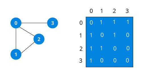
For example, we have a graph below.
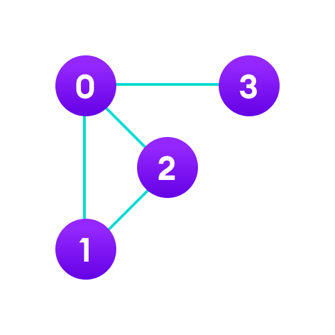
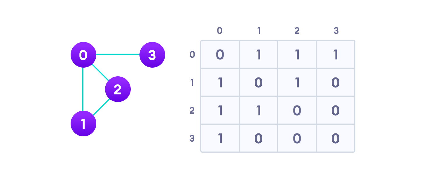
We can represent this graph in matrix form like below.
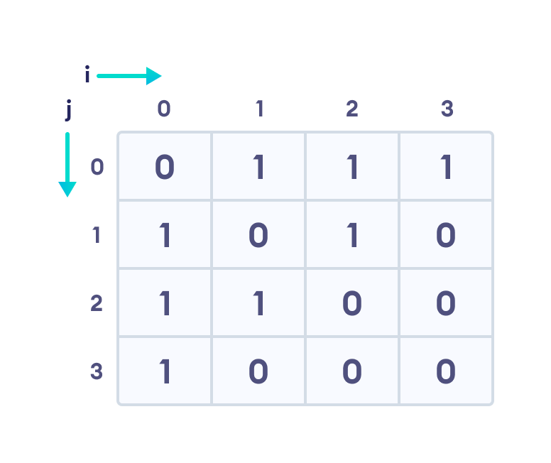
Each cell in the above table/matrix is represented as Aij, where i and j are vertices. The value of Aij is either 1 or 0 depending on whether there is an edge from vertex i to vertex j.
If there is a path from i to j, then the value of Aij is 1 otherwise its 0. For instance, there is a path from vertex 1 to vertex 2, so A12 is 1 and there is no path from vertex 1 to 3, so A13 is 0.
In case of undirected graphs, the matrix is symmetric about the diagonal because of every edge (i,j), there is also an edge (j,i).
Pros of Adjacency Matrix
- The basic operations like adding an edge, removing an edge, and checking whether there is an edge from vertex i to vertex j are extremely time efficient, constant time operations.
- If the graph is dense and the number of edges is large, an adjacency matrix should be the first choice. Even if the graph and the adjacency matrix is sparse, we can represent it using data structures for sparse matrices.
- The biggest advantage, however, comes from the use of matrices. The recent advances in hardware enable us to perform even expensive matrix operations on the GPU.
- By performing operations on the adjacent matrix, we can get important insights into the nature of the graph and the relationship between its vertices.
Cons of Adjacency Matrix
- The
VxVspace requirement of the adjacency matrix makes it a memory hog. Graphs out in the wild usually don't have too many connections and this is the major reason why adjacency lists are the better choice for most tasks. - While basic operations are easy, operations like
inEdgesandoutEdgesare expensive when using the adjacency matrix representation.
Adjacency Matrix Code in Python, Java, and C/C++
If you know how to create two-dimensional arrays, you also know how to create an adjacency matrix.
# Adjacency Matrix representation in Python


class Graph(object):

    # Initialize the matrix
    def __init__(self, size):
        self.adjMatrix = []
        for i in range(size):
            self.adjMatrix.append([0 for i in range(size)])
        self.size = size

    # Add edges
    def add_edge(self, v1, v2):
        if v1 == v2:
            print("Same vertex %d and %d" % (v1, v2))
        self.adjMatrix[v1][v2] = 1
        self.adjMatrix[v2][v1] = 1

    # Remove edges
    def remove_edge(self, v1, v2):
        if self.adjMatrix[v1][v2] == 0:
            print("No edge between %d and %d" % (v1, v2))
            return
        self.adjMatrix[v1][v2] = 0
        self.adjMatrix[v2][v1] = 0

    def __len__(self):
        return self.size

    # Print the matrix
    def print_matrix(self):
        for row in self.adjMatrix:
            for val in row:
                print('{:4}'.format(val)),
            print


def main():
    g = Graph(5)
    g.add_edge(0, 1)
    g.add_edge(0, 2)
    g.add_edge(1, 2)
    g.add_edge(2, 0)
    g.add_edge(2, 3)

    g.print_matrix()


if __name__ == '__main__':
    main()
// Adjacency Matrix representation in Java

public class Graph {
  private boolean adjMatrix[][];
  private int numVertices;

  // Initialize the matrix
  public Graph(int numVertices) {
    this.numVertices = numVertices;
    adjMatrix = new boolean[numVertices][numVertices];
  }

  // Add edges
  public void addEdge(int i, int j) {
    adjMatrix[i][j] = true;
    adjMatrix[j][i] = true;
  }

  // Remove edges
  public void removeEdge(int i, int j) {
    adjMatrix[i][j] = false;
    adjMatrix[j][i] = false;
  }

  // Print the matrix
  public String toString() {
    StringBuilder s = new StringBuilder();
    for (int i = 0; i < numVertices; i++) {
      s.append(i + ": ");
      for (boolean j : adjMatrix[i]) {
        s.append((j ? 1 : 0) + " ");
      }
      s.append("\n");
    }
    return s.toString();
  }

  public static void main(String args[]) {
    Graph g = new Graph(4);

    g.addEdge(0, 1);
    g.addEdge(0, 2);
    g.addEdge(1, 2);
    g.addEdge(2, 0);
    g.addEdge(2, 3);

    System.out.print(g.toString());
  }
}
// Adjacency Matrix representation in C

#include <stdio.h>
#define V 4

// Initialize the matrix to zero
void init(int arr[][V]) {
  int i, j;
  for (i = 0; i < V; i++)
    for (j = 0; j < V; j++)
      arr[i][j] = 0;
}

// Add edges
void addEdge(int arr[][V], int i, int j) {
  arr[i][j] = 1;
  arr[j][i] = 1;
}

// Print the matrix
void printAdjMatrix(int arr[][V]) {
  int i, j;

  for (i = 0; i < V; i++) {
    printf("%d: ", i);
    for (j = 0; j < V; j++) {
      printf("%d ", arr[i][j]);
    }
    printf("\n");
  }
}

int main() {
  int adjMatrix[V][V];

  init(adjMatrix);
  addEdge(adjMatrix, 0, 1);
  addEdge(adjMatrix, 0, 2);
  addEdge(adjMatrix, 1, 2);
  addEdge(adjMatrix, 2, 0);
  addEdge(adjMatrix, 2, 3);

  printAdjMatrix(adjMatrix);

  return 0;
}
// Adjacency Matrix representation in C++

#include <iostream>
using namespace std;

class Graph {
   private:
  bool** adjMatrix;
  int numVertices;

   public:
  // Initialize the matrix to zero
  Graph(int numVertices) {
    this->numVertices = numVertices;
    adjMatrix = new bool*[numVertices];
    for (int i = 0; i < numVertices; i++) {
      adjMatrix[i] = new bool[numVertices];
      for (int j = 0; j < numVertices; j++)
        adjMatrix[i][j] = false;
    }
  }

  // Add edges
  void addEdge(int i, int j) {
    adjMatrix[i][j] = true;
    adjMatrix[j][i] = true;
  }

  // Remove edges
  void removeEdge(int i, int j) {
    adjMatrix[i][j] = false;
    adjMatrix[j][i] = false;
  }

  // Print the martix
  void toString() {
    for (int i = 0; i < numVertices; i++) {
      cout << i << " : ";
      for (int j = 0; j < numVertices; j++)
        cout << adjMatrix[i][j] << " ";
      cout << "\n";
    }
  }

  ~Graph() {
    for (int i = 0; i < numVertices; i++)
      delete[] adjMatrix[i];
    delete[] adjMatrix;
  }
};

int main() {
  Graph g(4);

  g.addEdge(0, 1);
  g.addEdge(0, 2);
  g.addEdge(1, 2);
  g.addEdge(2, 0);
  g.addEdge(2, 3);

  g.toString();
}
Adjacency Matrix Applications
- Creating routing table in networks
- Navigation tasks
Adjacency List
An adjacency list represents a graph as an array of linked lists. The index of the array represents a vertex and each element in its linked list represents the other vertices that form an edge with the vertex.
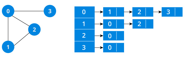
For example, we have a graph below.
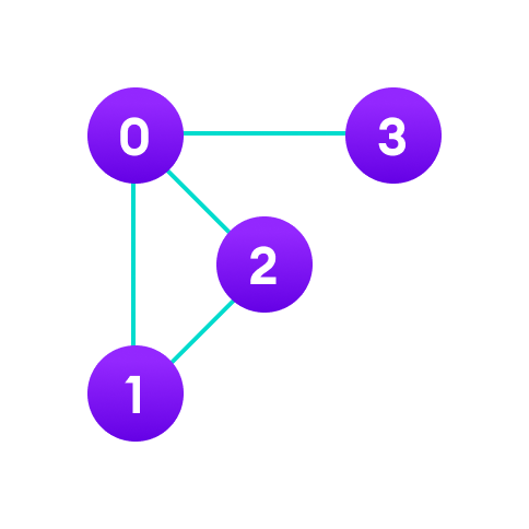
We can represent this graph in the form of a linked list on a computer as shown below.
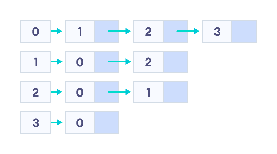
Here, 0, 1, 2, 3 are the vertices and each of them forms a linked list with all of its adjacent vertices. For instance, vertex 1 has two adjacent vertices 0 and 2. Therefore, 1 is linked with 0 and 2 in the figure above.
Pros of Adjacency List
- An adjacency list is efficient in terms of storage because we only need to store the values for the edges. For a sparse graph with millions of vertices and edges, this can mean a lot of saved space.
- It also helps to find all the vertices adjacent to a vertex easily.
Cons of Adjacency List
- Finding the adjacent list is not quicker than the adjacency matrix because all the connected nodes must be first explored to find them.
Adjacency List Structure
The simplest adjacency list needs a node data structure to store a vertex and a graph data structure to organize the nodes.
We stay close to the basic definition of a graph - a collection of vertices and edges {V, E}. For simplicity, we use an unlabeled graph as opposed to a labeled one i.e. the vertices are identified by their indices 0,1,2,3.
Let's dig into the data structures at play here.
struct node{
    int vertex;
    struct node* next;
};

struct Graph{
    int numVertices;
    struct node** adjLists;
};
Don't let the struct node** adjLists overwhelm you.
All we are saying is we want to store a pointer to struct node*. This is because we don't know how many vertices the graph will have and so we cannot create an array of Linked Lists at compile time.
Adjacency List C++
It is the same structure but by using the in-built list STL data structures of C++, we make the structure a bit cleaner. We are also able to abstract the details of the implementation.
class Graph{
    int numVertices;
    list<int> *adjLists;

  public:
    Graph(int V);
    void addEdge(int src, int dest);
};
Adjacency List Java
We use Java Collections to store the Array of Linked Lists.
class Graph{
    private int numVertices;
    private LinkedList<integer> adjLists[];
}
The type of LinkedList is determined by what data you want to store in it. For a labeled graph, you could store a dictionary instead of an Integer
Adjacency List Python
There is a reason Python gets so much love. A simple dictionary of vertices and its edges is a sufficient representation of a graph. You can make the vertex itself as complex as you want.
graph = {'A': set(['B', 'C']),
         'B': set(['A', 'D', 'E']),
         'C': set(['A', 'F']),
         'D': set(['B']),
         'E': set(['B', 'F']),
         'F': set(['C', 'E'])}
Adjacency List Code in Python, Java, and C/C++
# Adjascency List representation in Python


class AdjNode:
    def __init__(self, value):
        self.vertex = value
        self.next = None


class Graph:
    def __init__(self, num):
        self.V = num
        self.graph = [None] * self.V

    # Add edges
    def add_edge(self, s, d):
        node = AdjNode(d)
        node.next = self.graph[s]
        self.graph[s] = node

        node = AdjNode(s)
        node.next = self.graph[d]
        self.graph[d] = node

    # Print the graph
    def print_agraph(self):
        for i in range(self.V):
            print("Vertex " + str(i) + ":", end="")
            temp = self.graph[i]
            while temp:
                print(" -> {}".format(temp.vertex), end="")
                temp = temp.next
            print(" \n")


if __name__ == "__main__":
    V = 5

    # Create graph and edges
    graph = Graph(V)
    graph.add_edge(0, 1)
    graph.add_edge(0, 2)
    graph.add_edge(0, 3)
    graph.add_edge(1, 2)

    graph.print_agraph()
// Adjascency List representation in Java

import java.util.*;

class Graph {

  // Add edge
  static void addEdge(ArrayList<ArrayList<Integer>> am, int s, int d) {
    am.get(s).add(d);
    am.get(d).add(s);
  }

  public static void main(String[] args) {

    // Create the graph
    int V = 5;
    ArrayList<ArrayList<Integer>> am = new ArrayList<ArrayList<Integer>>(V);

    for (int i = 0; i < V; i++)
      am.add(new ArrayList<Integer>());

    // Add edges
    addEdge(am, 0, 1);
    addEdge(am, 0, 2);
    addEdge(am, 0, 3);
    addEdge(am, 1, 2);

    printGraph(am);
  }

  // Print the graph
  static void printGraph(ArrayList<ArrayList<Integer>> am) {
    for (int i = 0; i < am.size(); i++) {
      System.out.println("\nVertex " + i + ":");
      for (int j = 0; j < am.get(i).size(); j++) {
        System.out.print(" -> " + am.get(i).get(j));
      }
      System.out.println();
    }
  }
}
// Adjascency List representation in C

#include <stdio.h>
#include <stdlib.h>

struct node {
  int vertex;
  struct node* next;
};
struct node* createNode(int);

struct Graph {
  int numVertices;
  struct node** adjLists;
};

// Create a node
struct node* createNode(int v) {
  struct node* newNode = malloc(sizeof(struct node));
  newNode->vertex = v;
  newNode->next = NULL;
  return newNode;
}

// Create a graph
struct Graph* createAGraph(int vertices) {
  struct Graph* graph = malloc(sizeof(struct Graph));
  graph->numVertices = vertices;

  graph->adjLists = malloc(vertices * sizeof(struct node*));

  int i;
  for (i = 0; i < vertices; i++)
    graph->adjLists[i] = NULL;

  return graph;
}

// Add edge
void addEdge(struct Graph* graph, int s, int d) {
  // Add edge from s to d
  struct node* newNode = createNode(d);
  newNode->next = graph->adjLists[s];
  graph->adjLists[s] = newNode;

  // Add edge from d to s
  newNode = createNode(s);
  newNode->next = graph->adjLists[d];
  graph->adjLists[d] = newNode;
}

// Print the graph
void printGraph(struct Graph* graph) {
  int v;
  for (v = 0; v < graph->numVertices; v++) {
    struct node* temp = graph->adjLists[v];
    printf("\n Vertex %d\n: ", v);
    while (temp) {
      printf("%d -> ", temp->vertex);
      temp = temp->next;
    }
    printf("\n");
  }
}

int main() {
  struct Graph* graph = createAGraph(4);
  addEdge(graph, 0, 1);
  addEdge(graph, 0, 2);
  addEdge(graph, 0, 3);
  addEdge(graph, 1, 2);

  printGraph(graph);

  return 0;
}
// Adjascency List representation in C++

#include <bits/stdc++.h>
using namespace std;

// Add edge
void addEdge(vector<int> adj[], int s, int d) {
  adj[s].push_back(d);
  adj[d].push_back(s);
}

// Print the graph
void printGraph(vector<int> adj[], int V) {
  for (int d = 0; d < V; ++d) {
    cout << "\n Vertex "
       << d << ":";
    for (auto x : adj[d])
      cout << "-> " << x;
    printf("\n");
  }
}

int main() {
  int V = 5;

  // Create a graph
  vector<int> adj[V];

  // Add edges
  addEdge(adj, 0, 1);
  addEdge(adj, 0, 2);
  addEdge(adj, 0, 3);
  addEdge(adj, 1, 2);
  printGraph(adj, V);
}
Applications of Adjacency List
- It is faster to use adjacency lists for graphs having less number of edges.
Depth First Search (DFS)
Depth first Search or Depth first traversal is a recursive algorithm for searching all the vertices of a graph or tree data structure. Traversal means visiting all the nodes of a graph.
Depth First Search Algorithm
A standard DFS implementation puts each vertex of the graph into one of two categories:
- Visited
- Not Visited
The purpose of the algorithm is to mark each vertex as visited while avoiding cycles.
The DFS algorithm works as follows:
- Start by putting any one of the graph's vertices on top of a stack.
- Take the top item of the stack and add it to the visited list.
- Create a list of that vertex's adjacent nodes. Add the ones which aren't in the visited list to the top of the stack.
- Keep repeating steps 2 and 3 until the stack is empty.
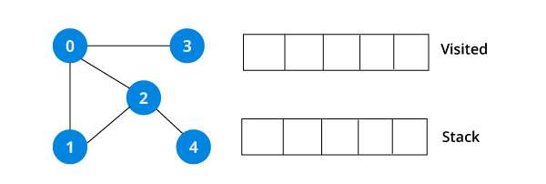
Depth First Search Example
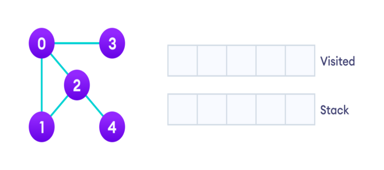
Let's see how the Depth First Search algorithm works with an example. We use an undirected graph with 5 vertices.
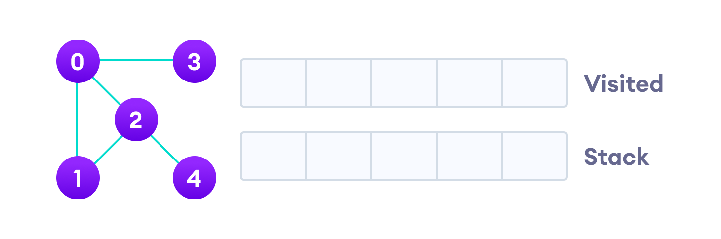
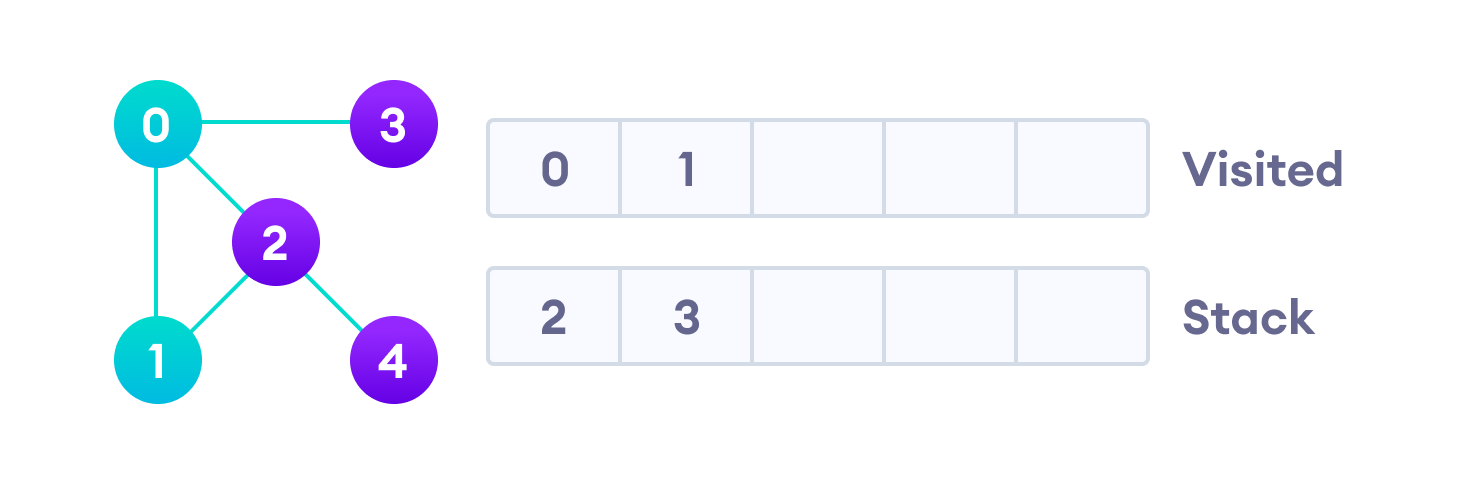
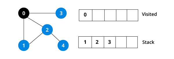
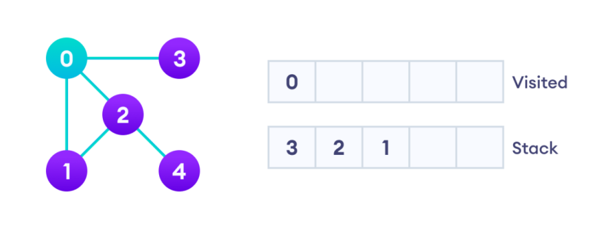
We start from vertex 0, the DFS algorithm starts by putting it in the Visited list and putting all its adjacent vertices in the stack.
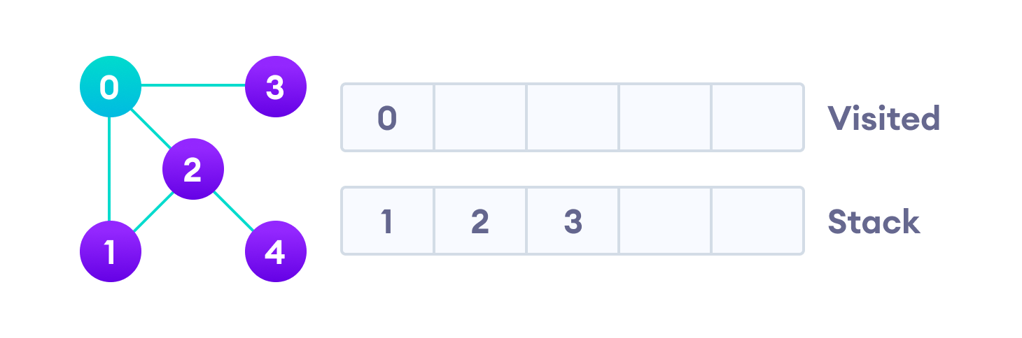
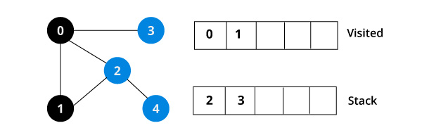
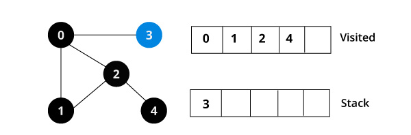
Next, we visit the element at the top of stack i.e. 1 and go to its adjacent nodes. Since 0 has already been visited, we visit 2 instead.
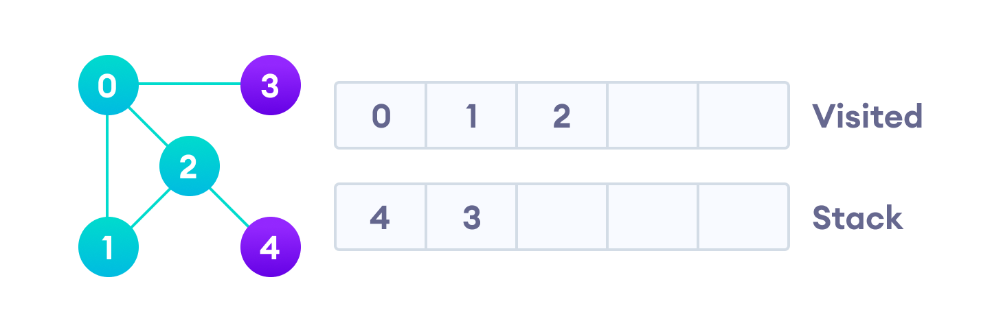
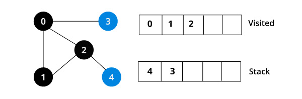
Vertex 2 has an unvisited adjacent vertex in 4, so we add that to the top of the stack and visit it.
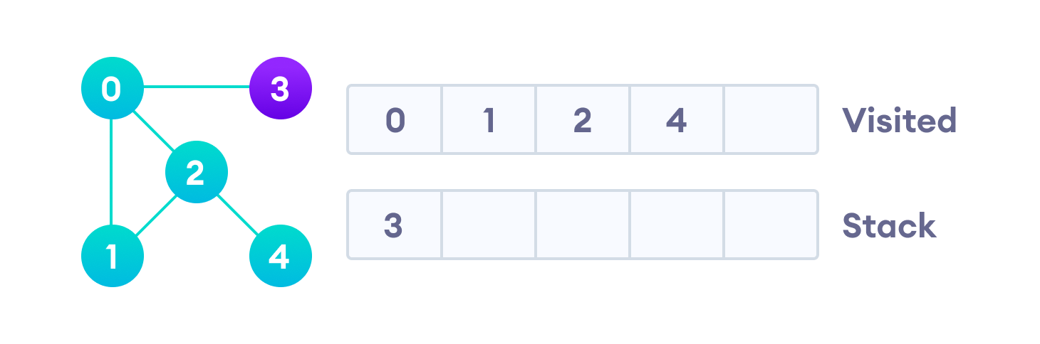
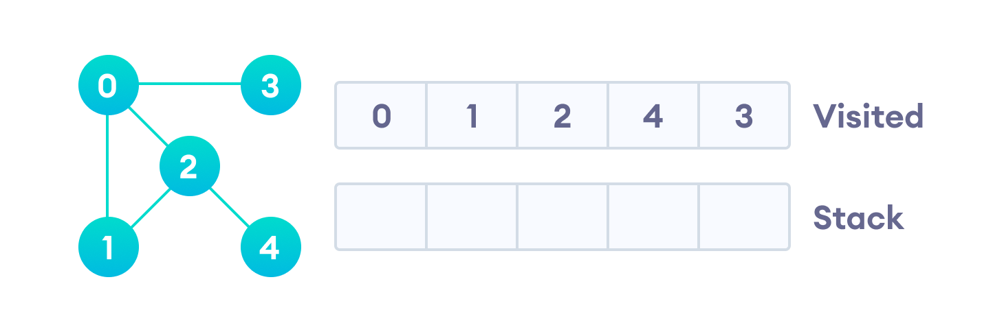
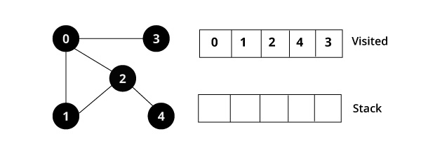
After we visit the last element 3, it doesn't have any unvisited adjacent nodes, so we have completed the Depth First Traversal of the graph.
DFS Pseudocode (recursive implementation)
The pseudocode for DFS is shown below. In the init() function, notice that we run the DFS function on every node. This is because the graph might have two different disconnected parts so to make sure that we cover every vertex, we can also run the DFS algorithm on every node.
DFS(G, u)
    u.visited = true
    for each v ∈ G.Adj[u]
        if v.visited == false
            DFS(G,v)

init() {
    For each u ∈ G
        u.visited = false
     For each u ∈ G
       DFS(G, u)
}
DFS Implementation in Python, Java and C/C++
The code for the Depth First Search Algorithm with an example is shown below. The code has been simplified so that we can focus on the algorithm rather than other details.
DFS Visualization: Don't just read about DFS, watch it happen live. See how each line of the algorithm works step-by-step with our new DSA visualizer. Try it yourself!
# DFS algorithm in Python


# DFS algorithm
def dfs(graph, start, visited=None):
    if visited is None:
        visited = set()
    visited.add(start)

    print(start)

    for next in graph[start] - visited:
        dfs(graph, next, visited)
    return visited


graph = {'0': set(['1', '2']),
         '1': set(['0', '3', '4']),
         '2': set(['0']),
         '3': set(['1']),
         '4': set(['2', '3'])}

dfs(graph, '0')
// DFS algorithm in Java

import java.util.*;

class Graph {
  private LinkedList<Integer> adjLists[];
  private boolean visited[];

  // Graph creation
  Graph(int vertices) {
    adjLists = new LinkedList[vertices];
    visited = new boolean[vertices];

    for (int i = 0; i < vertices; i++)
      adjLists[i] = new LinkedList<Integer>();
  }

  // Add edges
  void addEdge(int src, int dest) {
    adjLists[src].add(dest);
  }

  // DFS algorithm
  void DFS(int vertex) {
    visited[vertex] = true;
    System.out.print(vertex + " ");

    Iterator<Integer> ite = adjLists[vertex].listIterator();
    while (ite.hasNext()) {
      int adj = ite.next();
      if (!visited[adj])
        DFS(adj);
    }
  }

  public static void main(String args[]) {
    Graph g = new Graph(4);

    g.addEdge(0, 1);
    g.addEdge(0, 2);
    g.addEdge(1, 2);
    g.addEdge(2, 3);

    System.out.println("Following is Depth First Traversal");

    g.DFS(2);
  }
}
// DFS algorithm in C

#include <stdio.h>
#include <stdlib.h>

struct node {
  int vertex;
  struct node* next;
};

struct node* createNode(int v);

struct Graph {
  int numVertices;
  int* visited;

  // We need int** to store a two dimensional array.
  // Similary, we need struct node** to store an array of Linked lists
  struct node** adjLists;
};

// DFS algo
void DFS(struct Graph* graph, int vertex) {
  struct node* adjList = graph->adjLists[vertex];
  struct node* temp = adjList;

  graph->visited[vertex] = 1;
  printf("Visited %d \n", vertex);

  while (temp != NULL) {
    int connectedVertex = temp->vertex;

    if (graph->visited[connectedVertex] == 0) {
      DFS(graph, connectedVertex);
    }
    temp = temp->next;
  }
}

// Create a node
struct node* createNode(int v) {
  struct node* newNode = malloc(sizeof(struct node));
  newNode->vertex = v;
  newNode->next = NULL;
  return newNode;
}

// Create graph
struct Graph* createGraph(int vertices) {
  struct Graph* graph = malloc(sizeof(struct Graph));
  graph->numVertices = vertices;

  graph->adjLists = malloc(vertices * sizeof(struct node*));

  graph->visited = malloc(vertices * sizeof(int));

  int i;
  for (i = 0; i < vertices; i++) {
    graph->adjLists[i] = NULL;
    graph->visited[i] = 0;
  }
  return graph;
}

// Add edge
void addEdge(struct Graph* graph, int src, int dest) {
  // Add edge from src to dest
  struct node* newNode = createNode(dest);
  newNode->next = graph->adjLists[src];
  graph->adjLists[src] = newNode;

  // Add edge from dest to src
  newNode = createNode(src);
  newNode->next = graph->adjLists[dest];
  graph->adjLists[dest] = newNode;
}

// Print the graph
void printGraph(struct Graph* graph) {
  int v;
  for (v = 0; v < graph->numVertices; v++) {
    struct node* temp = graph->adjLists[v];
    printf("\n Adjacency list of vertex %d\n ", v);
    while (temp) {
      printf("%d -> ", temp->vertex);
      temp = temp->next;
    }
    printf("\n");
  }
}

int main() {
  struct Graph* graph = createGraph(4);
  addEdge(graph, 0, 1);
  addEdge(graph, 0, 2);
  addEdge(graph, 1, 2);
  addEdge(graph, 2, 3);

  printGraph(graph);

  DFS(graph, 2);

  return 0;
}
// DFS algorithm in C++

#include <iostream>
#include <list>
using namespace std;

class Graph {
  int numVertices;
  list<int> *adjLists;
  bool *visited;

   public:
  Graph(int V);
  void addEdge(int src, int dest);
  void DFS(int vertex);
};

// Initialize graph
Graph::Graph(int vertices) {
  numVertices = vertices;
  adjLists = new list<int>[vertices];
  visited = new bool[vertices];
}

// Add edges
void Graph::addEdge(int src, int dest) {
  adjLists[src].push_front(dest);
}

// DFS algorithm
void Graph::DFS(int vertex) {
  visited[vertex] = true;
  list<int> adjList = adjLists[vertex];

  cout << vertex << " ";

  list<int>::iterator i;
  for (i = adjList.begin(); i != adjList.end(); ++i)
    if (!visited[*i])
      DFS(*i);
}

int main() {
  Graph g(4);
  g.addEdge(0, 1);
  g.addEdge(0, 2);
  g.addEdge(1, 2);
  g.addEdge(2, 3);

  g.DFS(2);

  return 0;
}
Complexity of Depth First Search
The time complexity of the DFS algorithm is represented in the form of O(V + E), where V is the number of nodes and E is the number of edges.
The space complexity of the algorithm is O(V).
Application of DFS Algorithm
- For finding the path
- To test if the graph is bipartite
- For finding the strongly connected components of a graph
- For detecting cycles in a graph
Graph Data Stucture
A graph data structure is a collection of nodes that have data and are connected to other nodes.
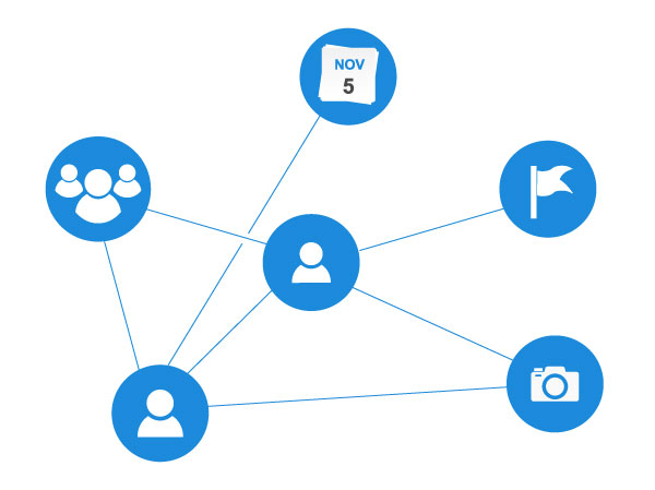
Let's try to understand this through an example. On facebook, everything is a node. That includes User, Photo, Album, Event, Group, Page, Comment, Story, Video, Link, Note...anything that has data is a node.
Every relationship is an edge from one node to another. Whether you post a photo, join a group, like a page, etc., a new edge is created for that relationship.
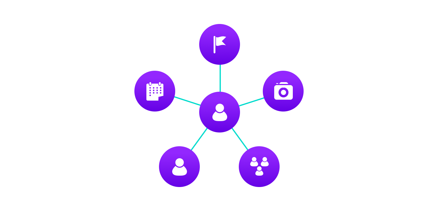
All of facebook is then a collection of these nodes and edges. This is because facebook uses a graph data structure to store its data.
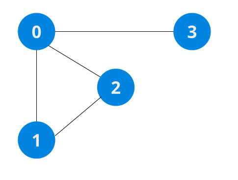
More precisely, a graph is a data structure (V, E) that consists of
- A collection of vertices V
- A collection of edges E, represented as ordered pairs of vertices (u,v)
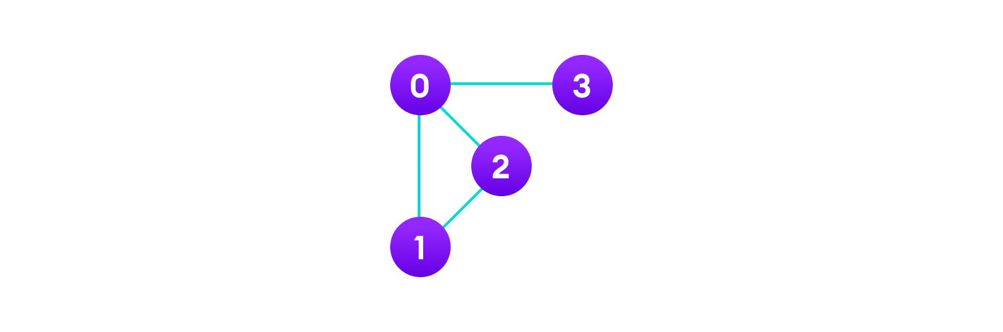
In the graph,
V = {0, 1, 2, 3}
E = {(0,1), (0,2), (0,3), (1,2)}
G = {V, E}
Graph Terminology
- Adjacency: A vertex is said to be adjacent to another vertex if there is an edge connecting them. Vertices 2 and 3 are not adjacent because there is no edge between them.
- Path: A sequence of edges that allows you to go from vertex A to vertex B is called a path. 0-1, 1-2 and 0-2 are paths from vertex 0 to vertex 2.
- Directed Graph: A graph in which an edge (u,v) doesn't necessarily mean that there is an edge (v, u) as well. The edges in such a graph are represented by arrows to show the direction of the edge.
Graph Representation
Graphs are commonly represented in two ways:
1. Adjacency Matrix
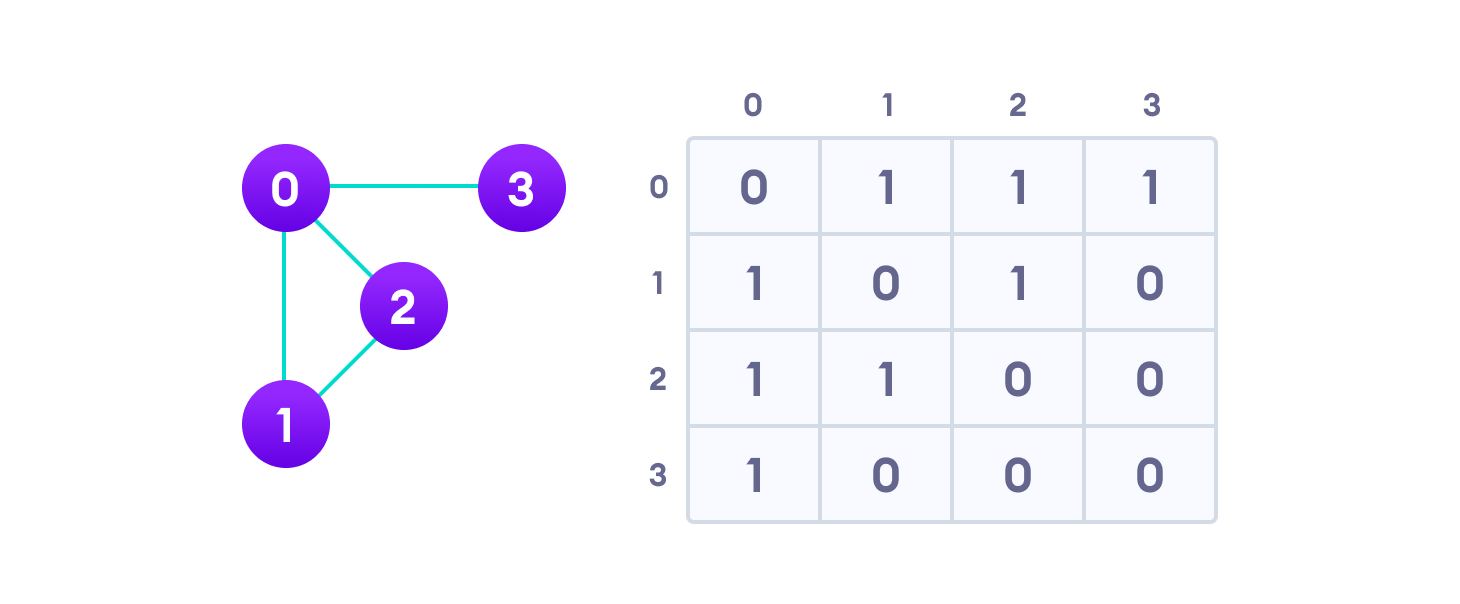
An adjacency matrix is a 2D array of V x V vertices. Each row and column represent a vertex.
If the value of any element a[i][j] is 1, it represents that there is an edge connecting vertex i and vertex j.
The adjacency matrix for the graph we created above is
Since it is an undirected graph, for edge (0,2), we also need to mark edge (2,0); making the adjacency matrix symmetric about the diagonal.
Edge lookup(checking if an edge exists between vertex A and vertex B) is extremely fast in adjacency matrix representation but we have to reserve space for every possible link between all vertices(V x V), so it requires more space.
2. Adjacency List
An adjacency list represents a graph as an array of linked lists.
The index of the array represents a vertex and each element in its linked list represents the other vertices that form an edge with the vertex.
The adjacency list for the graph we made in the first example is as follows:
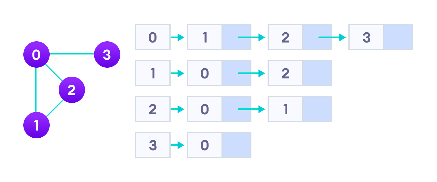
An adjacency list is efficient in terms of storage because we only need to store the values for the edges. For a graph with millions of vertices, this can mean a lot of saved space.
Graph Operations
The most common graph operations are:
- Check if the element is present in the graph
- Graph Traversal
- Add elements(vertex, edges) to graph
- Finding the path from one vertex to another
Binary Search Tree(BST)
Binary search tree is a data structure that quickly allows us to maintain a sorted list of numbers.
- It is called a binary tree because each tree node has a maximum of two children.
- It is called a search tree because it can be used to search for the presence of a number in
O(log(n))time.
The properties that separate a binary search tree from a regular binary tree is
- All nodes of left subtree are less than the root node
- All nodes of right subtree are more than the root node
- Both subtrees of each node are also BSTs i.e. they have the above two properties
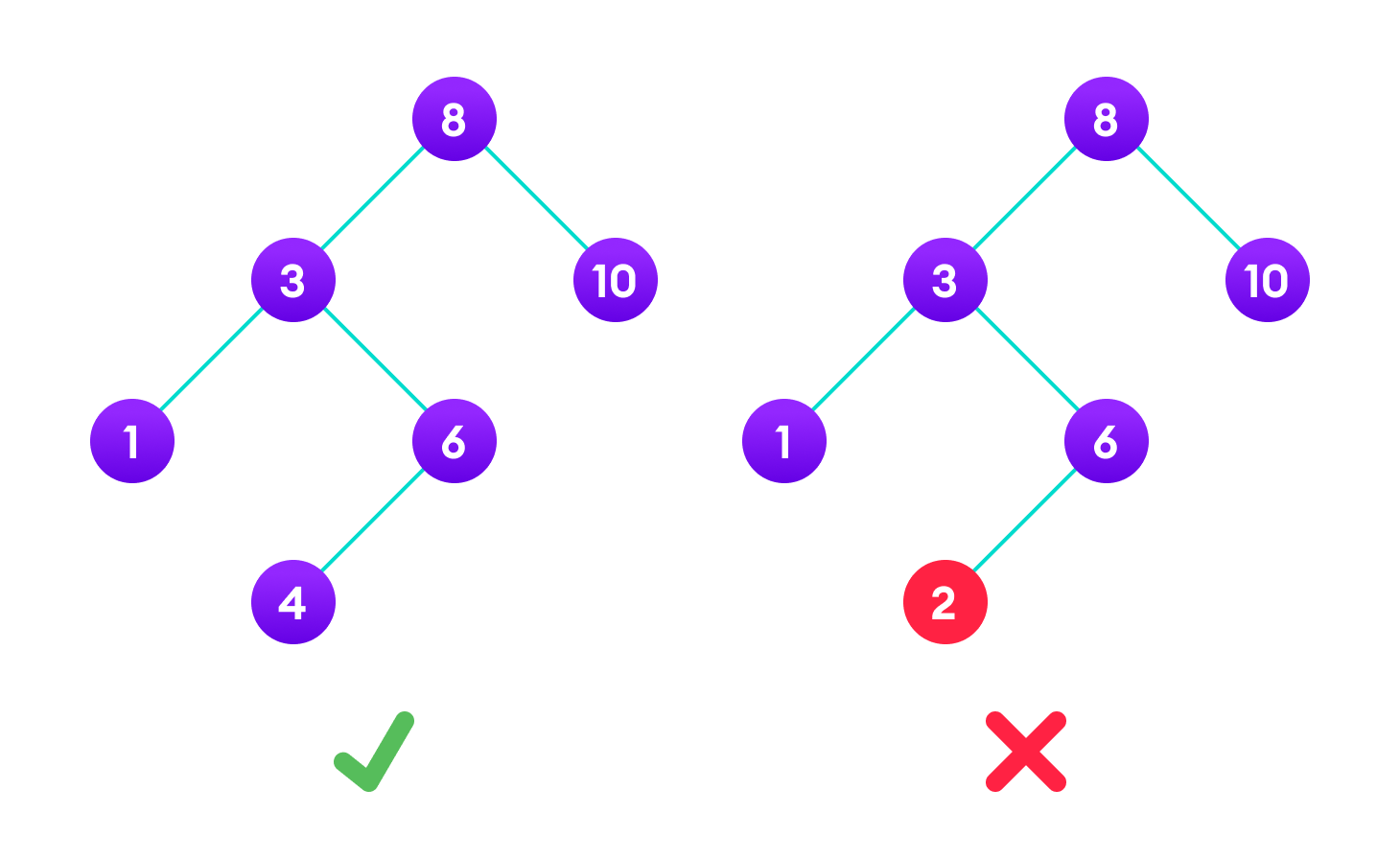
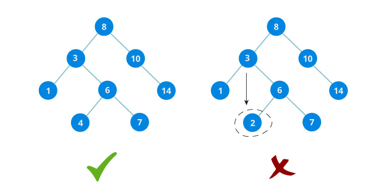
The binary tree on the right isn't a binary search tree because the right subtree of the node "3" contains a value smaller than it.
There are two basic operations that you can perform on a binary search tree:
Search Operation
The algorithm depends on the property of BST that if each left subtree has values below root and each right subtree has values above the root.
If the value is below the root, we can say for sure that the value is not in the right subtree; we need to only search in the left subtree and if the value is above the root, we can say for sure that the value is not in the left subtree; we need to only search in the right subtree.
Algorithm:
If root == NULL
    return NULL;
If number == root->data
    return root->data;
If number < root->data
    return search(root->left)
If number > root->data
    return search(root->right)
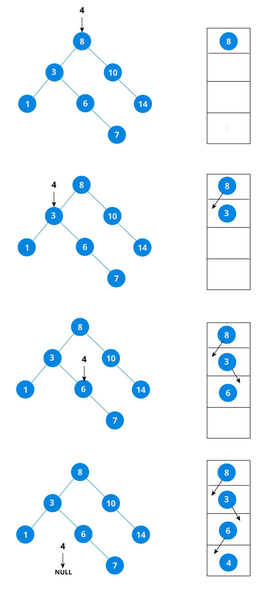
Let us try to visualize this with a diagram.
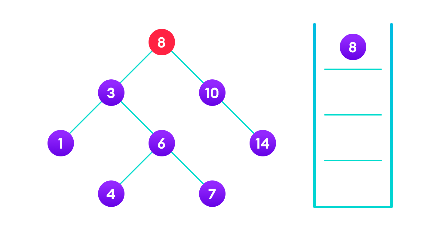
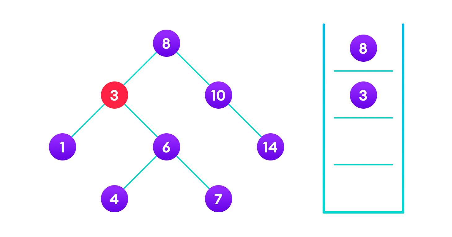
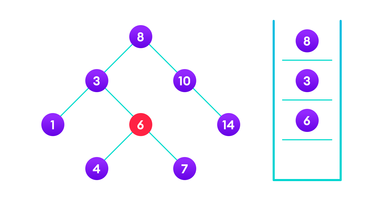
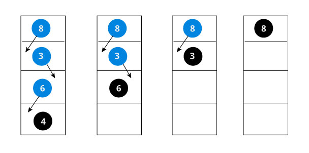
If the value is found, we return the value so that it gets propagated in each recursion step as shown in the image below.
If you might have noticed, we have called return search(struct node*) four times. When we return either the new node or NULL, the value gets returned again and again until search(root) returns the final result.
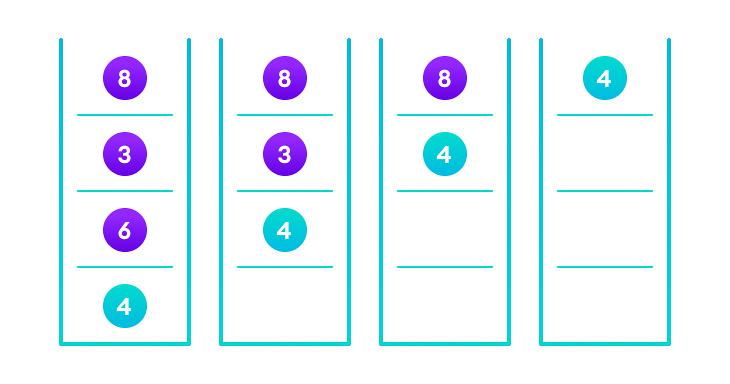
If the value is not found, we eventually reach the left or right child of a leaf node which is NULL and it gets propagated and returned.
Insert Operation
Inserting a value in the correct position is similar to searching because we try to maintain the rule that the left subtree is lesser than root and the right subtree is larger than root.
We keep going to either right subtree or left subtree depending on the value and when we reach a point left or right subtree is null, we put the new node there.
Algorithm:
If node == NULL
    return createNode(data)
if (data < node->data)
    node->left  = insert(node->left, data);
else if (data > node->data)
    node->right = insert(node->right, data);
return node;
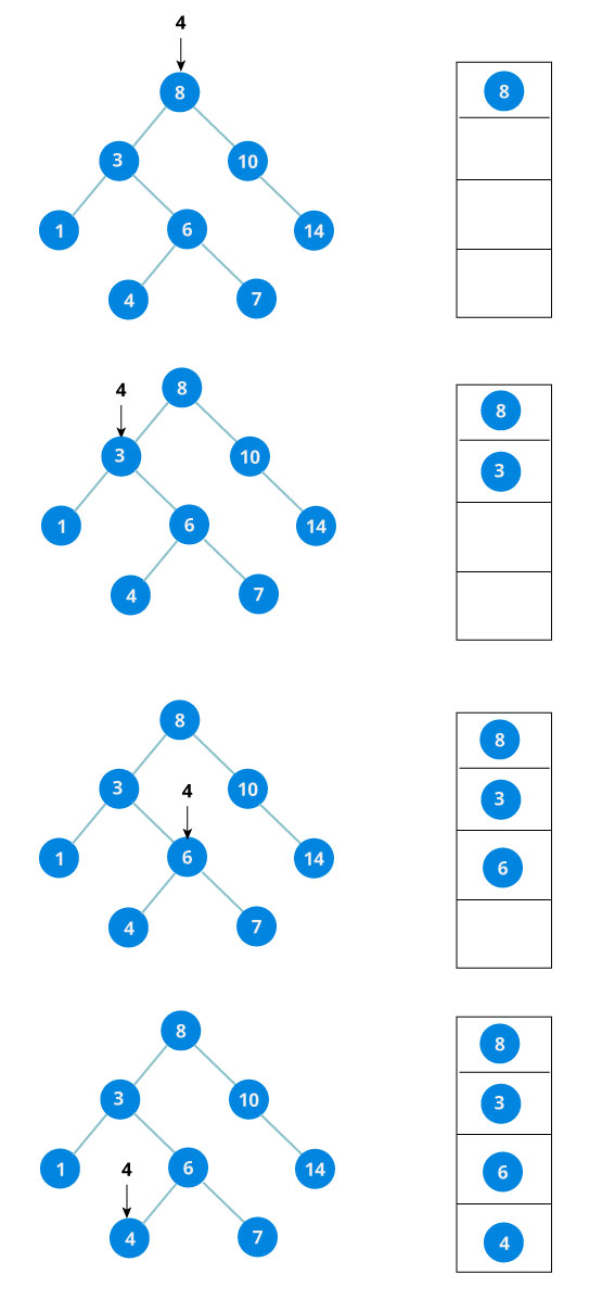
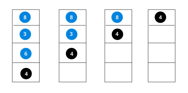
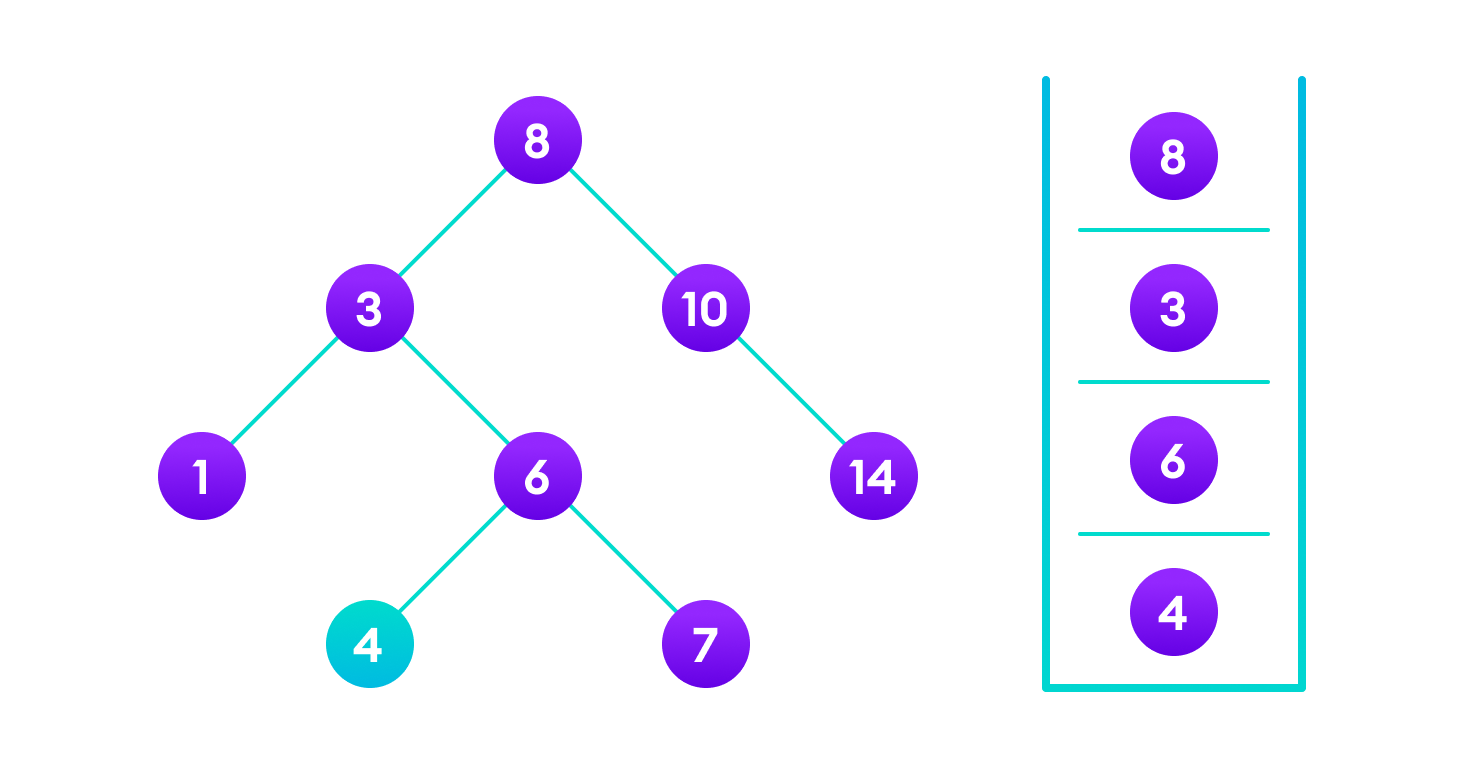
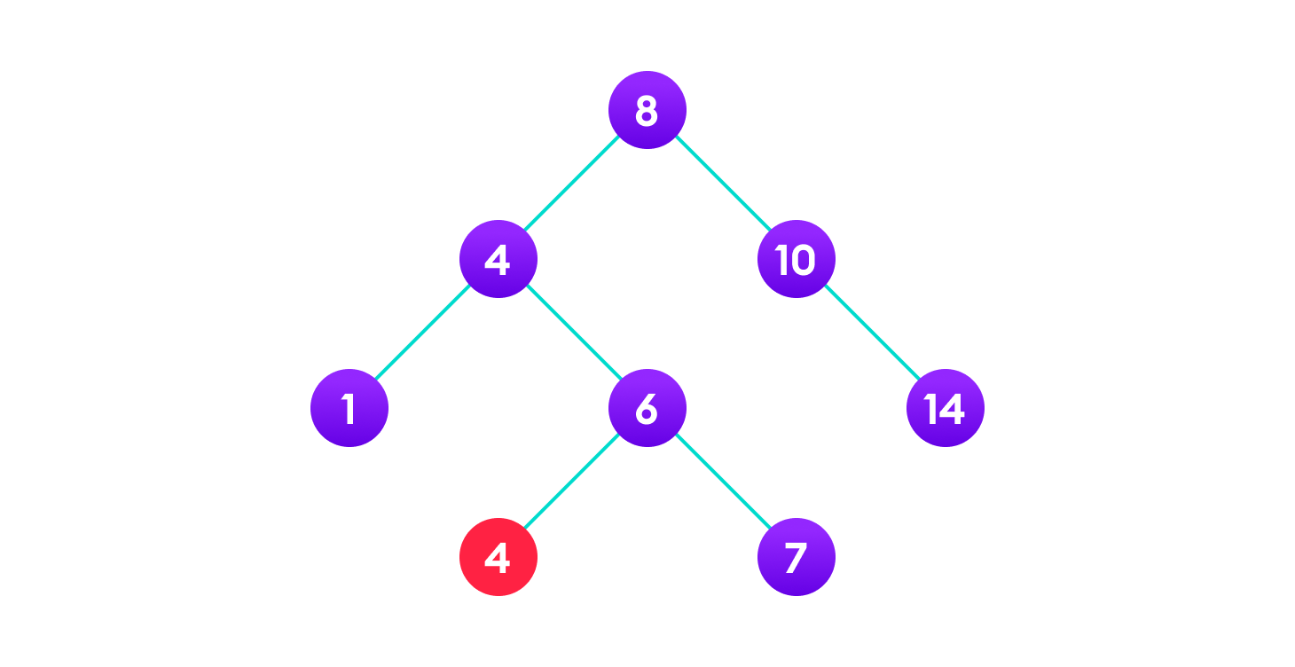
The algorithm isn't as simple as it looks. Let's try to visualize how we add a number to an existing BST.
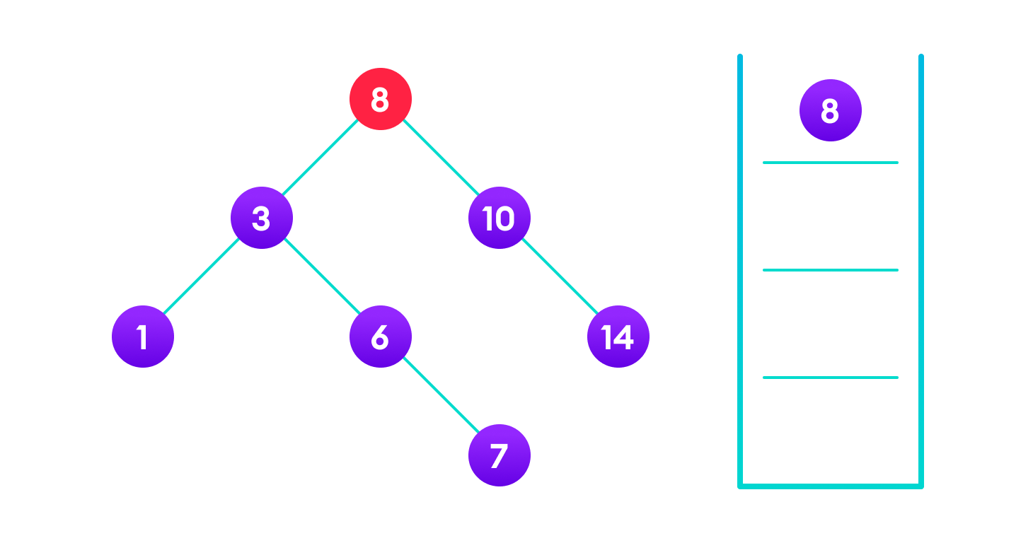
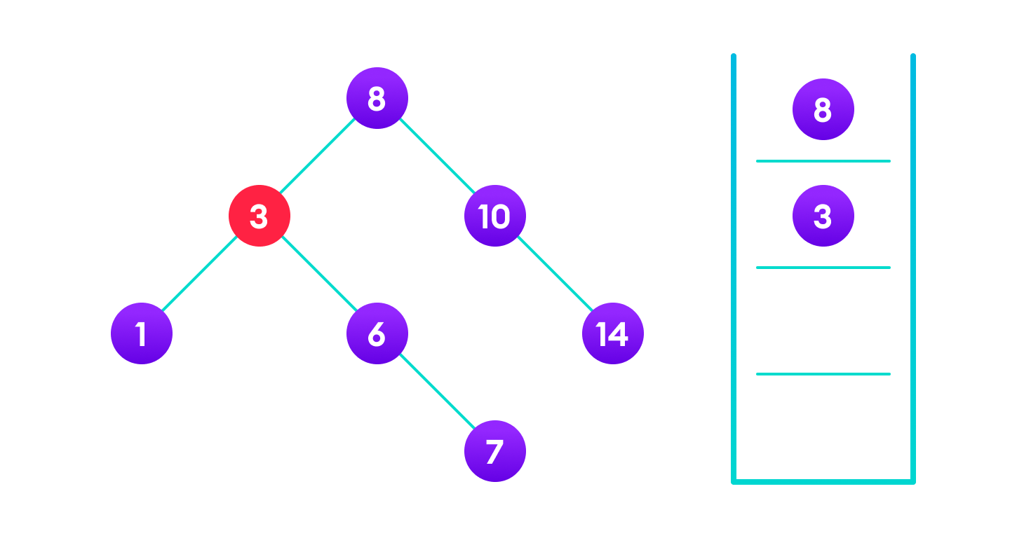
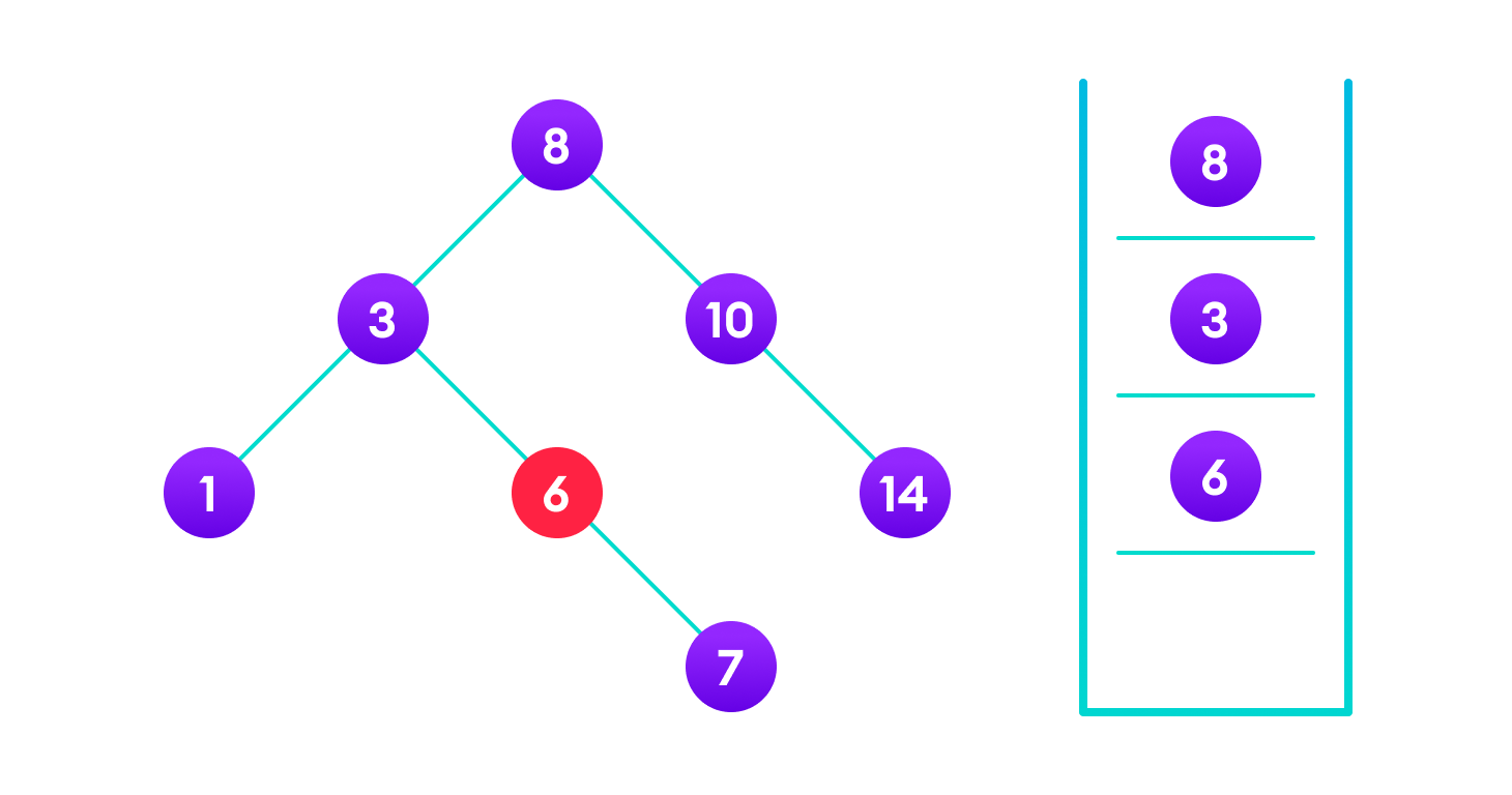
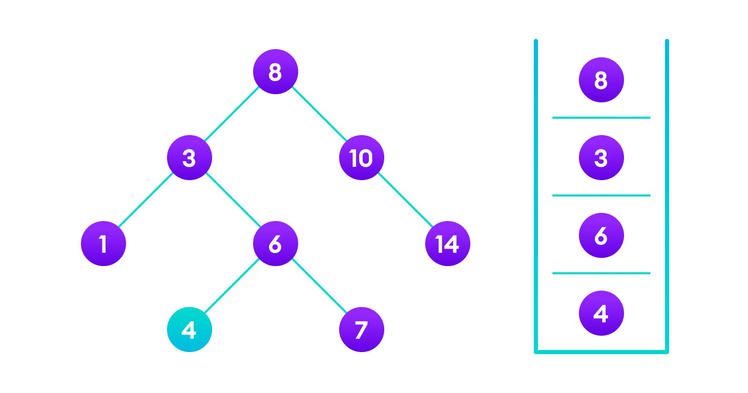
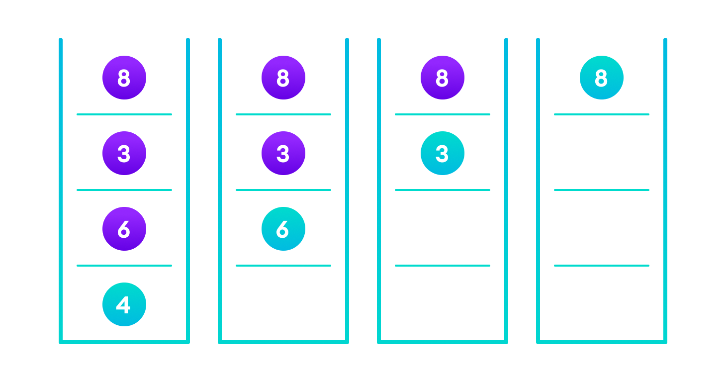
We have attached the node but we still have to exit from the function without doing any damage to the rest of the tree. This is where the return node; at the end comes in handy. In the case of NULL, the newly created node is returned and attached to the parent node, otherwise the same node is returned without any change as we go up until we return to the root.
This makes sure that as we move back up the tree, the other node connections aren't changed.
Deletion Operation
There are three cases for deleting a node from a binary search tree.
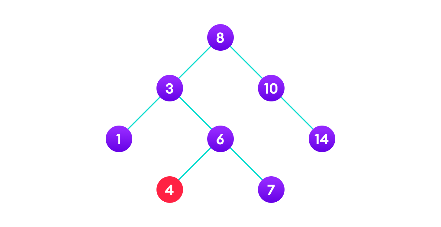
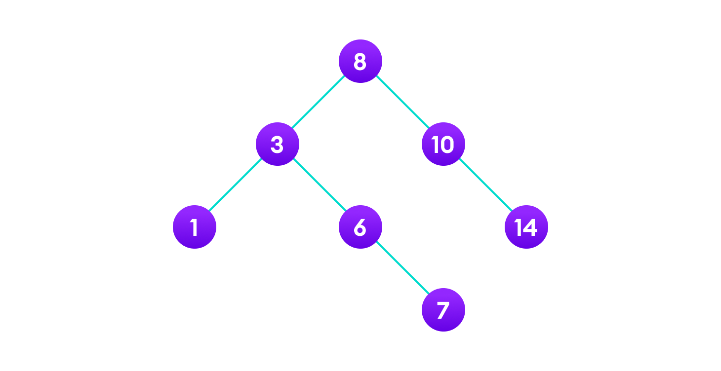
Case I
In the first case, the node to be deleted is the leaf node. In such a case, simply delete the node from the tree.
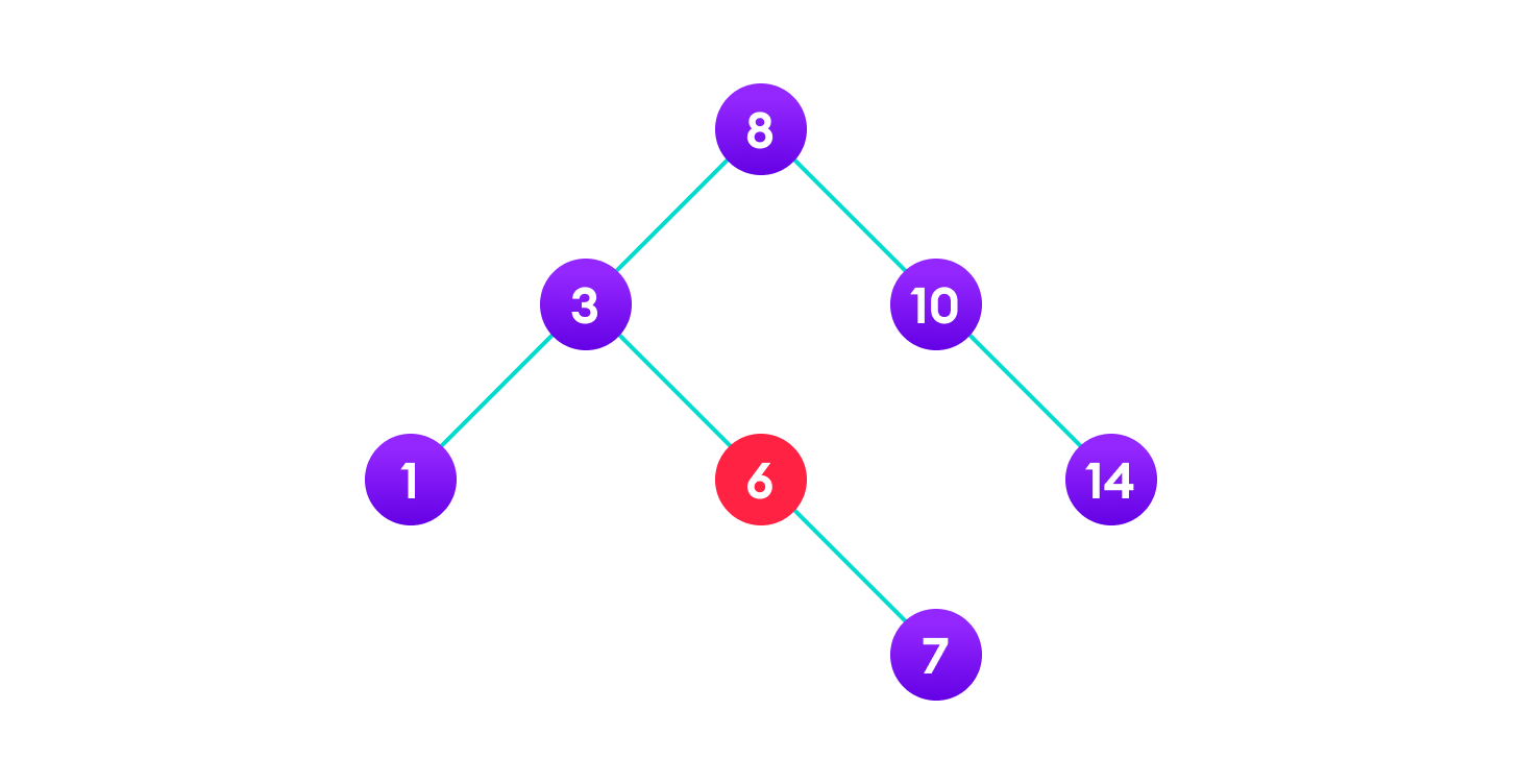
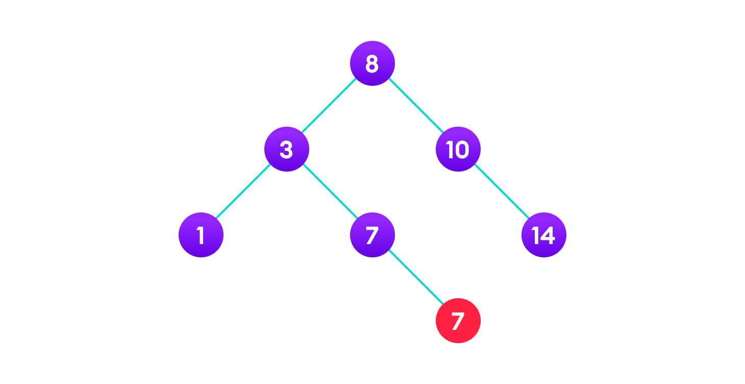
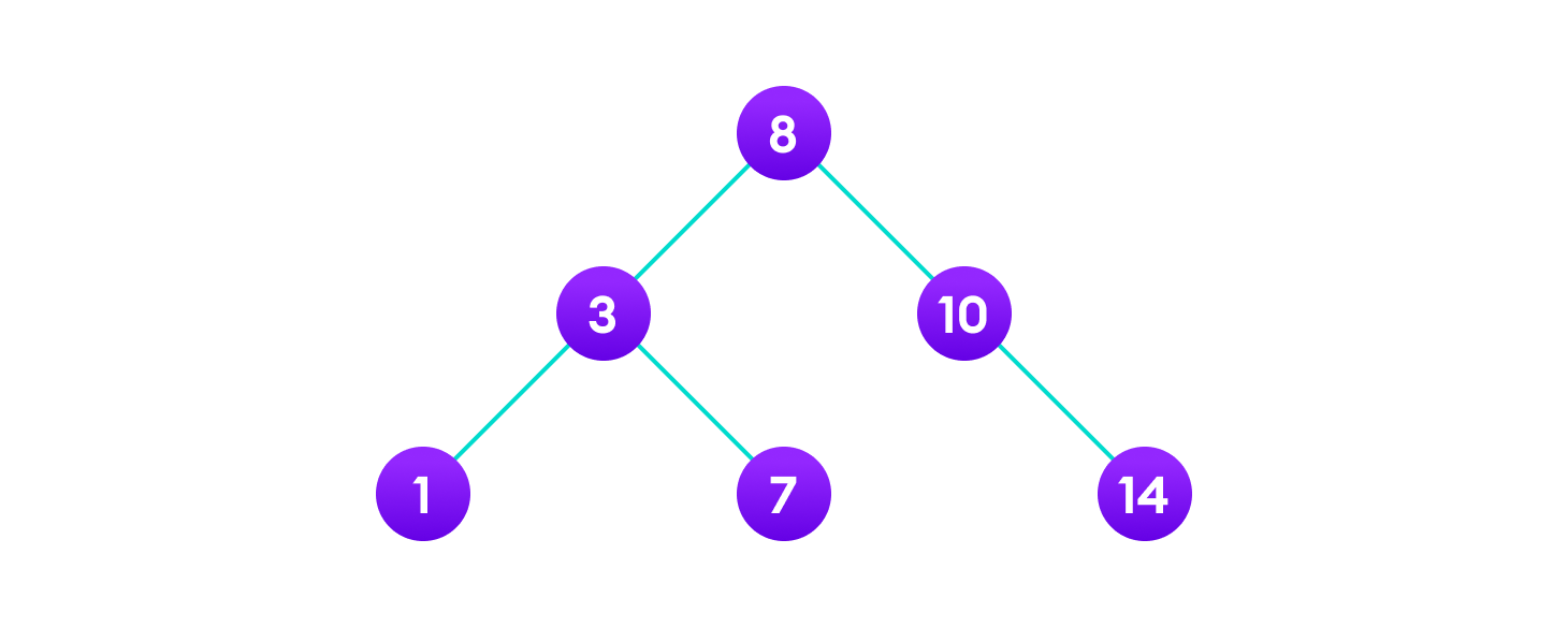
Case II
In the second case, the node to be deleted lies has a single child node. In such a case follow the steps below:
- Replace that node with its child node.
- Remove the child node from its original position.
Case III
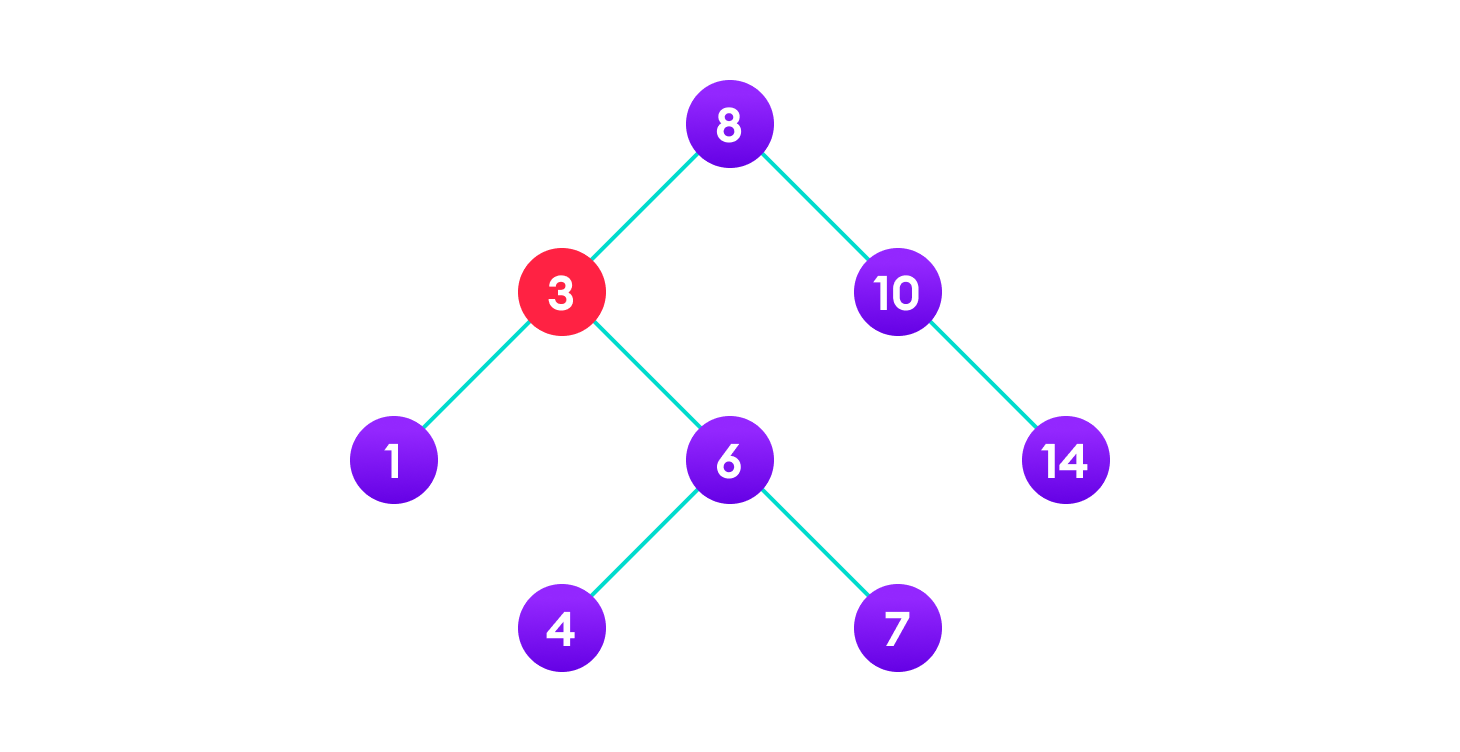
In the third case, the node to be deleted has two children. In such a case follow the steps below:
- Get the inorder successor of that node.
- Replace the node with the inorder successor.
- Remove the inorder successor from its original position.
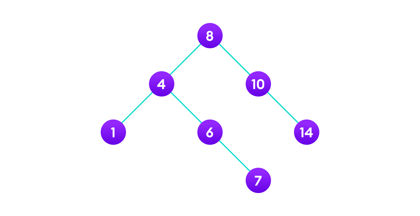
Python, Java and C/C++ Examples
# Binary Search Tree operations in Python


# Create a node
class Node:
    def __init__(self, key):
        self.key = key
        self.left = None
        self.right = None


# Inorder traversal
def inorder(root):
    if root is not None:
        # Traverse left
        inorder(root.left)

        # Traverse root
        print(str(root.key) + "->", end=' ')

        # Traverse right
        inorder(root.right)


# Insert a node
def insert(node, key):

    # Return a new node if the tree is empty
    if node is None:
        return Node(key)

    # Traverse to the right place and insert the node
    if key < node.key:
        node.left = insert(node.left, key)
    else:
        node.right = insert(node.right, key)

    return node


# Find the inorder successor
def minValueNode(node):
    current = node

    # Find the leftmost leaf
    while(current.left is not None):
        current = current.left

    return current


# Deleting a node
def deleteNode(root, key):

    # Return if the tree is empty
    if root is None:
        return root

    # Find the node to be deleted
    if key < root.key:
        root.left = deleteNode(root.left, key)
    elif(key > root.key):
        root.right = deleteNode(root.right, key)
    else:
        # If the node is with only one child or no child
        if root.left is None:
            temp = root.right
            root = None
            return temp

        elif root.right is None:
            temp = root.left
            root = None
            return temp

        # If the node has two children,
        # place the inorder successor in position of the node to be deleted
        temp = minValueNode(root.right)

        root.key = temp.key

        # Delete the inorder successor
        root.right = deleteNode(root.right, temp.key)

    return root


root = None
root = insert(root, 8)
root = insert(root, 3)
root = insert(root, 1)
root = insert(root, 6)
root = insert(root, 7)
root = insert(root, 10)
root = insert(root, 14)
root = insert(root, 4)

print("Inorder traversal: ", end=' ')
inorder(root)

print("\nDelete 10")
root = deleteNode(root, 10)
print("Inorder traversal: ", end=' ')
inorder(root)
// Binary Search Tree operations in Java

class BinarySearchTree {
  class Node {
    int key;
    Node left, right;

    public Node(int item) {
      key = item;
      left = right = null;
    }
  }

  Node root;

  BinarySearchTree() {
    root = null;
  }

  void insert(int key) {
    root = insertKey(root, key);
  }

  // Insert key in the tree
  Node insertKey(Node root, int key) {
    // Return a new node if the tree is empty
    if (root == null) {
      root = new Node(key);
      return root;
    }

    // Traverse to the right place and insert the node
    if (key < root.key)
      root.left = insertKey(root.left, key);
    else if (key > root.key)
      root.right = insertKey(root.right, key);

    return root;
  }

  void inorder() {
    inorderRec(root);
  }

  // Inorder Traversal
  void inorderRec(Node root) {
    if (root != null) {
      inorderRec(root.left);
      System.out.print(root.key + " -> ");
      inorderRec(root.right);
    }
  }

  void deleteKey(int key) {
    root = deleteRec(root, key);
  }

  Node deleteRec(Node root, int key) {
    // Return if the tree is empty
    if (root == null)
      return root;

    // Find the node to be deleted
    if (key < root.key)
      root.left = deleteRec(root.left, key);
    else if (key > root.key)
      root.right = deleteRec(root.right, key);
    else {
      // If the node is with only one child or no child
      if (root.left == null)
        return root.right;
      else if (root.right == null)
        return root.left;

      // If the node has two children
      // Place the inorder successor in position of the node to be deleted
      root.key = minValue(root.right);

      // Delete the inorder successor
      root.right = deleteRec(root.right, root.key);
    }

    return root;
  }

  // Find the inorder successor
  int minValue(Node root) {
    int minv = root.key;
    while (root.left != null) {
      minv = root.left.key;
      root = root.left;
    }
    return minv;
  }

  // Driver Program to test above functions
  public static void main(String[] args) {
    BinarySearchTree tree = new BinarySearchTree();

    tree.insert(8);
    tree.insert(3);
    tree.insert(1);
    tree.insert(6);
    tree.insert(7);
    tree.insert(10);
    tree.insert(14);
    tree.insert(4);

    System.out.print("Inorder traversal: ");
    tree.inorder();

    System.out.println("\n\nAfter deleting 10");
    tree.deleteKey(10);
    System.out.print("Inorder traversal: ");
    tree.inorder();
  }
}
// Binary Search Tree operations in C

#include <stdio.h>
#include <stdlib.h>

struct node {
  int key;
  struct node *left, *right;
};

// Create a node
struct node *newNode(int item) {
  struct node *temp = (struct node *)malloc(sizeof(struct node));
  temp->key = item;
  temp->left = temp->right = NULL;
  return temp;
}

// Inorder Traversal
void inorder(struct node *root) {
  if (root != NULL) {
    // Traverse left
    inorder(root->left);

    // Traverse root
    printf("%d -> ", root->key);

    // Traverse right
    inorder(root->right);
  }
}

// Insert a node
struct node *insert(struct node *node, int key) {
  // Return a new node if the tree is empty
  if (node == NULL) return newNode(key);

  // Traverse to the right place and insert the node
  if (key < node->key)
    node->left = insert(node->left, key);
  else
    node->right = insert(node->right, key);

  return node;
}

// Find the inorder successor
struct node *minValueNode(struct node *node) {
  struct node *current = node;

  // Find the leftmost leaf
  while (current && current->left != NULL)
    current = current->left;

  return current;
}

// Deleting a node
struct node *deleteNode(struct node *root, int key) {
  // Return if the tree is empty
  if (root == NULL) return root;

  // Find the node to be deleted
  if (key < root->key)
    root->left = deleteNode(root->left, key);
  else if (key > root->key)
    root->right = deleteNode(root->right, key);

  else {
    // If the node is with only one child or no child
    if (root->left == NULL) {
      struct node *temp = root->right;
      free(root);
      return temp;
    } else if (root->right == NULL) {
      struct node *temp = root->left;
      free(root);
      return temp;
    }

    // If the node has two children
    struct node *temp = minValueNode(root->right);

    // Place the inorder successor in position of the node to be deleted
    root->key = temp->key;

    // Delete the inorder successor
    root->right = deleteNode(root->right, temp->key);
  }
  return root;
}

// Driver code
int main() {
  struct node *root = NULL;
  root = insert(root, 8);
  root = insert(root, 3);
  root = insert(root, 1);
  root = insert(root, 6);
  root = insert(root, 7);
  root = insert(root, 10);
  root = insert(root, 14);
  root = insert(root, 4);

  printf("Inorder traversal: ");
  inorder(root);

  printf("\nAfter deleting 10\n");
  root = deleteNode(root, 10);
  printf("Inorder traversal: ");
  inorder(root);
}
// Binary Search Tree operations in C++

#include <iostream>
using namespace std;

struct node {
  int key;
  struct node *left, *right;
};

// Create a node
struct node *newNode(int item) {
  struct node *temp = (struct node *)malloc(sizeof(struct node));
  temp->key = item;
  temp->left = temp->right = NULL;
  return temp;
}

// Inorder Traversal
void inorder(struct node *root) {
  if (root != NULL) {
    // Traverse left
    inorder(root->left);

    // Traverse root
    cout << root->key << " -> ";

    // Traverse right
    inorder(root->right);
  }
}

// Insert a node
struct node *insert(struct node *node, int key) {
  // Return a new node if the tree is empty
  if (node == NULL) return newNode(key);

  // Traverse to the right place and insert the node
  if (key < node->key)
    node->left = insert(node->left, key);
  else
    node->right = insert(node->right, key);

  return node;
}

// Find the inorder successor
struct node *minValueNode(struct node *node) {
  struct node *current = node;

  // Find the leftmost leaf
  while (current && current->left != NULL)
    current = current->left;

  return current;
}

// Deleting a node
struct node *deleteNode(struct node *root, int key) {
  // Return if the tree is empty
  if (root == NULL) return root;

  // Find the node to be deleted
  if (key < root->key)
    root->left = deleteNode(root->left, key);
  else if (key > root->key)
    root->right = deleteNode(root->right, key);
  else {
    // If the node is with only one child or no child
    if (root->left == NULL) {
      struct node *temp = root->right;
      free(root);
      return temp;
    } else if (root->right == NULL) {
      struct node *temp = root->left;
      free(root);
      return temp;
    }

    // If the node has two children
    struct node *temp = minValueNode(root->right);

    // Place the inorder successor in position of the node to be deleted
    root->key = temp->key;

    // Delete the inorder successor
    root->right = deleteNode(root->right, temp->key);
  }
  return root;
}

// Driver code
int main() {
  struct node *root = NULL;
  root = insert(root, 8);
  root = insert(root, 3);
  root = insert(root, 1);
  root = insert(root, 6);
  root = insert(root, 7);
  root = insert(root, 10);
  root = insert(root, 14);
  root = insert(root, 4);

  cout << "Inorder traversal: ";
  inorder(root);

  cout << "\nAfter deleting 10\n";
  root = deleteNode(root, 10);
  cout << "Inorder traversal: ";
  inorder(root);
}
Binary Search Tree Complexities
Time Complexity
| Operation | Best Case Complexity | Average Case Complexity | Worst Case Complexity |
| Search | O(log n) | O(log n) | O(n) |
| Insertion | O(log n) | O(log n) | O(n) |
| Deletion | O(log n) | O(log n) | O(n) |
Here, n is the number of nodes in the tree.
Space Complexity
The space complexity for all the operations is O(n).
Binary Search Tree Applications
- In multilevel indexing in the database
- For dynamic sorting
- For managing virtual memory areas in Unix kernel
Tree Traversal - inorder, preorder and postorder
Traversing a tree means visiting every node in the tree. You might, for instance, want to add all the values in the tree or find the largest one. For all these operations, you will need to visit each node of the tree.
Linear data structures like arrays, stacks, queues, and linked list have only one way to read the data. But a hierarchical data structure like a tree can be traversed in different ways.
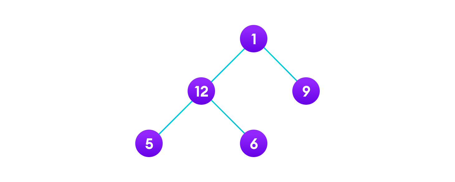
Let's think about how we can read the elements of the tree in the image shown above.
Starting from top, Left to right
1 -> 12 -> 5 -> 6 -> 9
Starting from bottom, Left to right
5 -> 6 -> 12 -> 9 -> 1
Although this process is somewhat easy, it doesn't respect the hierarchy of the tree, only the depth of the nodes.
Instead, we use traversal methods that take into account the basic structure of a tree i.e.
struct node {
    int data;
    struct node* left;
    struct node* right;
}
The struct node pointed to by left and right might have other left and right children so we should think of them as sub-trees instead of sub-nodes.
According to this structure, every tree is a combination of
- A node carrying data
- Two subtrees
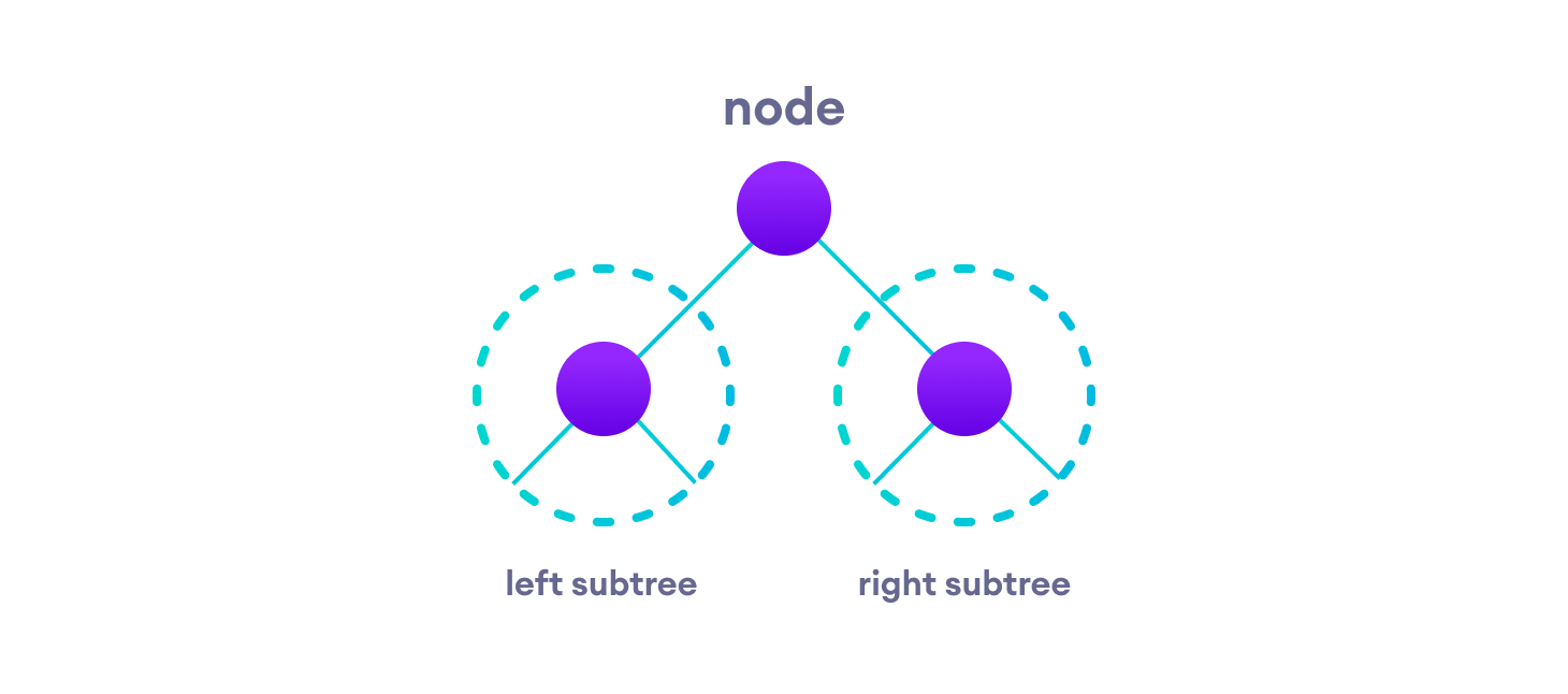
Remember that our goal is to visit each node, so we need to visit all the nodes in the subtree, visit the root node and visit all the nodes in the right subtree as well.
Depending on the order in which we do this, there can be three types of traversal.
Inorder traversal
- First, visit all the nodes in the left subtree
- Then the root node
- Visit all the nodes in the right subtree
inorder(root->left)
display(root->data)
inorder(root->right)
Preorder traversal
- Visit root node
- Visit all the nodes in the left subtree
- Visit all the nodes in the right subtree
display(root->data)
preorder(root->left)
preorder(root->right)
Postorder traversal
- Visit all the nodes in the left subtree
- Visit all the nodes in the right subtree
- Visit the root node
postorder(root->left)
postorder(root->right)
display(root->data)
Let's visualize in-order traversal. We start from the root node.
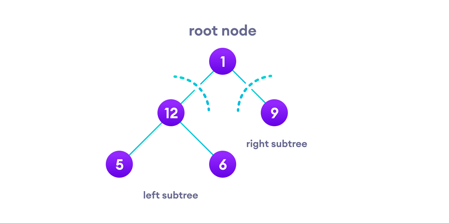
We traverse the left subtree first. We also need to remember to visit the root node and the right subtree when this tree is done.
Let's put all this in a stack so that we remember.
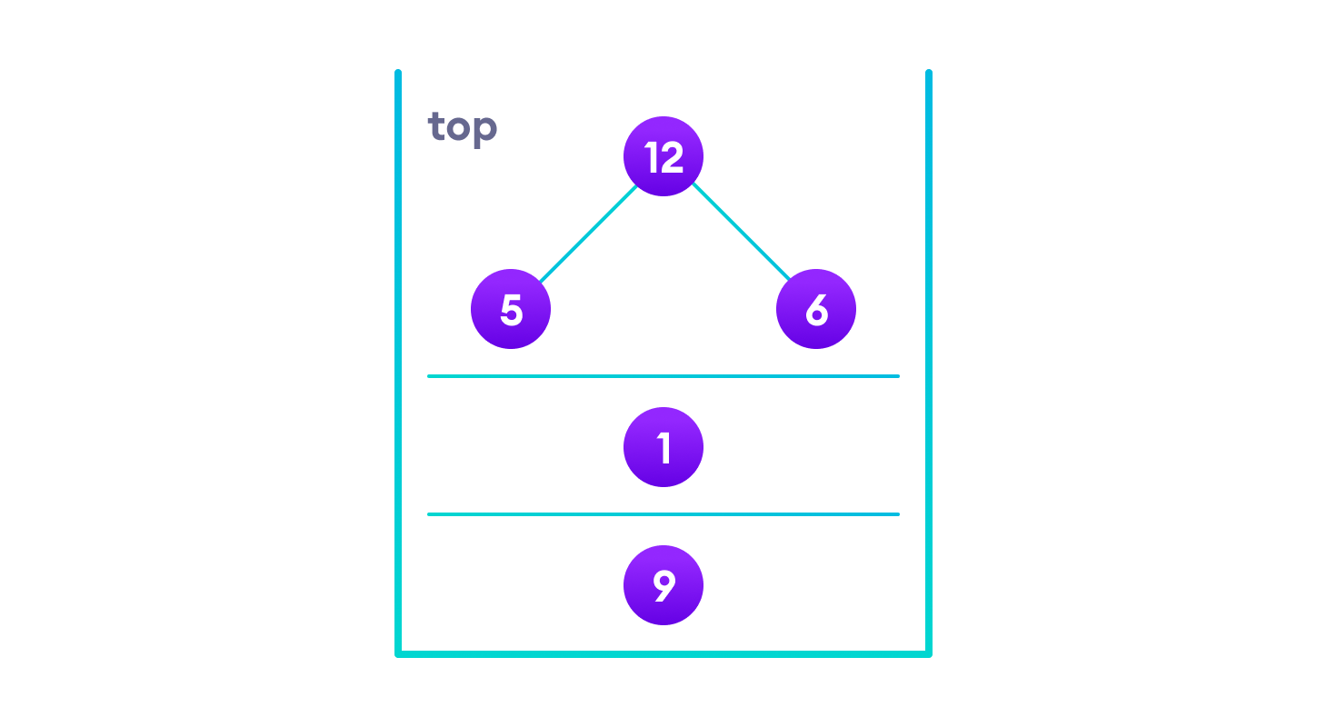
Now we traverse to the subtree pointed on the TOP of the stack.
Again, we follow the same rule of inorder
Left subtree -> root -> right subtree
After traversing the left subtree, we are left with
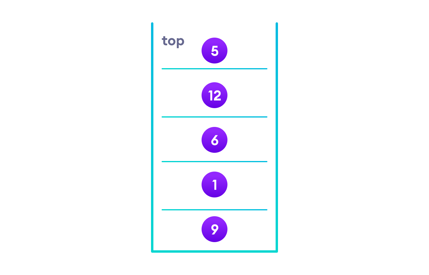
Since the node "5" doesn't have any subtrees, we print it directly. After that we print its parent "12" and then the right child "6".
Putting everything on a stack was helpful because now that the left-subtree of the root node has been traversed, we can print it and go to the right subtree.
After going through all the elements, we get the inorder traversal as
5 -> 12 -> 6 -> 1 -> 9
We don't have to create the stack ourselves because recursion maintains the correct order for us.
Python, Java and C/C++ Examples
# Tree traversal in Python


class Node:
    def __init__(self, item):
        self.left = None
        self.right = None
        self.val = item


def inorder(root):

    if root:
        # Traverse left
        inorder(root.left)
        # Traverse root
        print(str(root.val) + "->", end='')
        # Traverse right
        inorder(root.right)


def postorder(root):

    if root:
        # Traverse left
        postorder(root.left)
        # Traverse right
        postorder(root.right)
        # Traverse root
        print(str(root.val) + "->", end='')


def preorder(root):

    if root:
        # Traverse root
        print(str(root.val) + "->", end='')
        # Traverse left
        preorder(root.left)
        # Traverse right
        preorder(root.right)


root = Node(1)
root.left = Node(2)
root.right = Node(3)
root.left.left = Node(4)
root.left.right = Node(5)

print("Inorder traversal ")
inorder(root)

print("\nPreorder traversal ")
preorder(root)

print("\nPostorder traversal ")
postorder(root)
// Tree traversal in Java

class Node {
  int item;
  Node left, right;

  public Node(int key) {
  item = key;
  left = right = null;
  }
}

class BinaryTree {
  // Root of Binary Tree
  Node root;

  BinaryTree() {
  root = null;
  }

  void postorder(Node node) {
  if (node == null)
    return;

  // Traverse left
  postorder(node.left);
  // Traverse right
  postorder(node.right);
  // Traverse root
  System.out.print(node.item + "->");
  }

  void inorder(Node node) {
  if (node == null)
    return;

  // Traverse left
  inorder(node.left);
  // Traverse root
  System.out.print(node.item + "->");
  // Traverse right
  inorder(node.right);
  }

  void preorder(Node node) {
  if (node == null)
    return;

  // Traverse root
  System.out.print(node.item + "->");
  // Traverse left
  preorder(node.left);
  // Traverse right
  preorder(node.right);
  }

  public static void main(String[] args) {
  BinaryTree tree = new BinaryTree();
  tree.root = new Node(1);
  tree.root.left = new Node(12);
  tree.root.right = new Node(9);
  tree.root.left.left = new Node(5);
  tree.root.left.right = new Node(6);

  System.out.println("Inorder traversal");
  tree.inorder(tree.root);

  System.out.println("\nPreorder traversal ");
  tree.preorder(tree.root);

  System.out.println("\nPostorder traversal");
  tree.postorder(tree.root);
  }
}
// Tree traversal in C

#include <stdio.h>
#include <stdlib.h>

struct node {
  int item;
  struct node* left;
  struct node* right;
};

// Inorder traversal
void inorderTraversal(struct node* root) {
  if (root == NULL) return;
  inorderTraversal(root->left);
  printf("%d ->", root->item);
  inorderTraversal(root->right);
}

// preorderTraversal traversal
void preorderTraversal(struct node* root) {
  if (root == NULL) return;
  printf("%d ->", root->item);
  preorderTraversal(root->left);
  preorderTraversal(root->right);
}

// postorderTraversal traversal
void postorderTraversal(struct node* root) {
  if (root == NULL) return;
  postorderTraversal(root->left);
  postorderTraversal(root->right);
  printf("%d ->", root->item);
}

// Create a new Node
struct node* createNode(value) {
  struct node* newNode = malloc(sizeof(struct node));
  newNode->item = value;
  newNode->left = NULL;
  newNode->right = NULL;

  return newNode;
}

// Insert on the left of the node
struct node* insertLeft(struct node* root, int value) {
  root->left = createNode(value);
  return root->left;
}

// Insert on the right of the node
struct node* insertRight(struct node* root, int value) {
  root->right = createNode(value);
  return root->right;
}

int main() {
  struct node* root = createNode(1);
  insertLeft(root, 12);
  insertRight(root, 9);

  insertLeft(root->left, 5);
  insertRight(root->left, 6);

  printf("Inorder traversal \n");
  inorderTraversal(root);

  printf("\nPreorder traversal \n");
  preorderTraversal(root);

  printf("\nPostorder traversal \n");
  postorderTraversal(root);
}
// Tree traversal in C++

#include <iostream>
using namespace std;

struct Node {
  int data;
  struct Node *left, *right;
  Node(int data) {
    this->data = data;
    left = right = NULL;
  }
};

// Preorder traversal
void preorderTraversal(struct Node* node) {
  if (node == NULL)
    return;

  cout << node->data << "->";
  preorderTraversal(node->left);
  preorderTraversal(node->right);
}

// Postorder traversal
void postorderTraversal(struct Node* node) {
  if (node == NULL)
    return;

  postorderTraversal(node->left);
  postorderTraversal(node->right);
  cout << node->data << "->";
}

// Inorder traversal
void inorderTraversal(struct Node* node) {
  if (node == NULL)
    return;

  inorderTraversal(node->left);
  cout << node->data << "->";
  inorderTraversal(node->right);
}

int main() {
  struct Node* root = new Node(1);
  root->left = new Node(12);
  root->right = new Node(9);
  root->left->left = new Node(5);
  root->left->right = new Node(6);

  cout << "Inorder traversal ";
  inorderTraversal(root);

  cout << "\nPreorder traversal ";
  preorderTraversal(root);

  cout << "\nPostorder traversal ";
  postorderTraversal(root);
  return 0;
}