
Getting Started with DSA
Data Structures and Algorithms (DSA) form the foundation of problem-solving in computer science. Mastering DSA helps you write efficient and optimized code.
Though concepts remain the same across languages, your choice of language can shape the learning experience.
Let's explore how to get started with DSA in different languages and the advantages each one offers.
C++ is often the go-to choice for those diving deep into DSA. Here's why many prefer it:
Low-Level Control: Unlike higher-level languages, C++ provides direct access to memory and system resources, enabling you to understand the underlying mechanics of how data structures and algorithms operate, which is excellent for learning DSA.
Efficiency: C++ allows us to write highly optimized code, which is crucial when working on large-scale problems.
To start with DSA in C++, you just need to set up the C++ environment on your device.
To do so, visit Getting Started with C++.
C is often preferred by those looking to build a deep understanding of how data structures work at a low level. Here's why:
Minimal Abstraction: C has minimal abstractions, so we have direct control over memory and data manipulation. This makes it easier to understand how data structures like arrays, linked lists, and trees are implemented under the hood.
Pointer Mastery: C's use of pointers provides hands-on experience with memory addresses, which is critical when working with dynamic data structures like linked lists, trees, and graphs.
To start with DSA in C, you just need to set up the C environment on your device.
To do so, visit Getting Started with C.
Java is another popular language for learning DSA, especially for beginners who prefer object-oriented programming (OOP). Reasons to choose Java:
Robustness and Security: Java handles memory management automatically through garbage collection, making it easier for beginners to focus on solving problems rather than managing resources.
Community Support: With a large community, there's plenty of documentation, tutorials, and resources available to get you started with DSA in Java.
To start with DSA in Java, you just need to set up the Java environment on your device.
To do so, visit Getting Started with Java.
Python is a favorite among beginners for its simplicity and readability. Here is why it is preferred for learning DSA.
Easy Syntax: Python's syntax is clean and concise, which makes learning DSA concepts less intimidating. You can focus on solving the algorithm without worrying about the language's complexity.
Dynamically Typed: Python doesn't require explicit data types, making writing and testing code easier.
To start with DSA in Python, you just need to set up the Python environment on your device.
To do so, visit Getting Started With Python.
JavaScript is primarily known as a language for web development, but it's also used to learn DSA. Here is why:
Ease of Use: JavaScript can run directly in the browser, which means you can write and test DSA problems without setting up complex environments. This is ideal for quick learning and experimentation.
Versatility: JavaScript's ability to run in the browser and on the server (via Node.js) makes it accessible and easy to test DSA concepts online.
To start with DSA in JavaScript, you just need to set up the JavaScript environment on your device.
To do so, visit Getting Started With JavaScript.
Regardless of your chosen language, the key is mastering the core concepts and practicing regularly.
Each language offers unique tools and approaches that can help you gain a deeper understanding of DSA. Start small, build your skills gradually, and apply what you learn through consistent problem-solving.
Strongly Connected Components
A strongly connected component is the portion of a directed graph in which there is a path from each vertex to another vertex. It is applicable only on a directed graph.
For example:
Let us take the graph below.
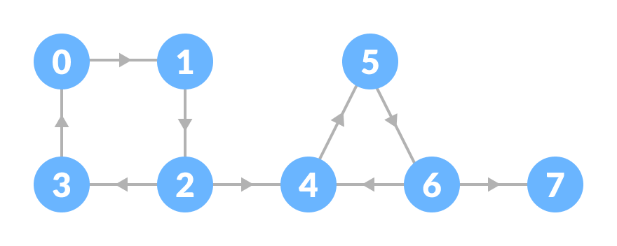
The strongly connected components of the above graph are:
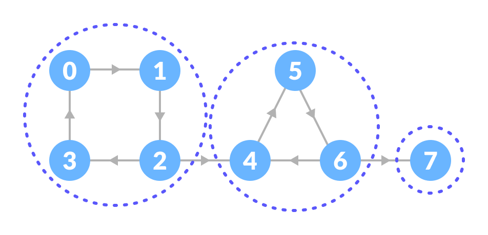
You can observe that in the first strongly connected component, every vertex can reach the other vertex through the directed path.
These components can be found using Kosaraju's Algorithm.
Kosaraju's Algorithm
Kosaraju's Algorithm is based on the depth-first search algorithm implemented twice.
Three steps are involved.
- Perform a depth first search on the whole graph.
Let us start from vertex-0, visit all of its child vertices, and mark the visited vertices as done. If a vertex leads to an already visited vertex, then push this vertex to the stack.
For example: Starting from vertex-0, go to vertex-1, vertex-2, and then to vertex-3. Vertex-3 leads to already visited vertex-0, so push the source vertex (ie. vertex-3) into the stack.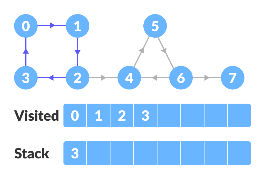
DFS on the graph
Go to the previous vertex (vertex-2) and visit its child vertices i.e. vertex-4, vertex-5, vertex-6 and vertex-7 sequentially. Since there is nowhere to go from vertex-7, push it into the stack.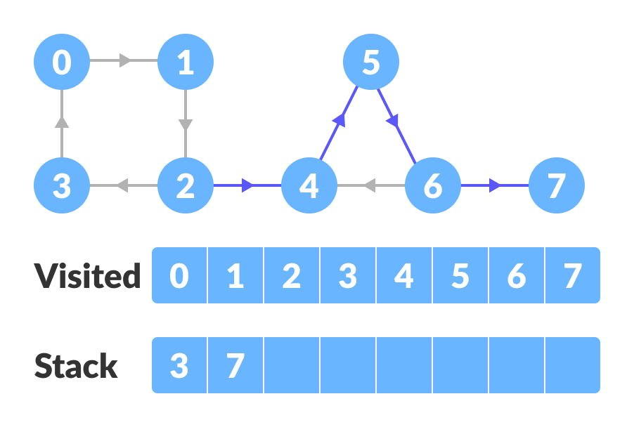
DFS on the graph
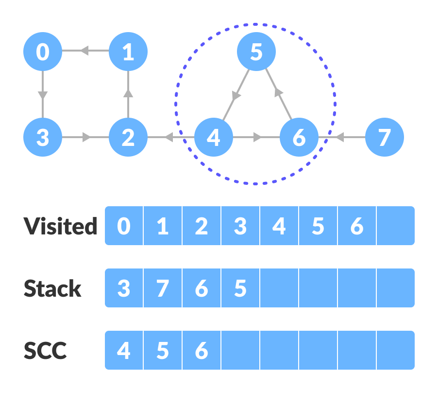
Go to the previous vertex (vertex-6) and visit its child vertices. But, all of its child vertices are visited, so push it into the stack.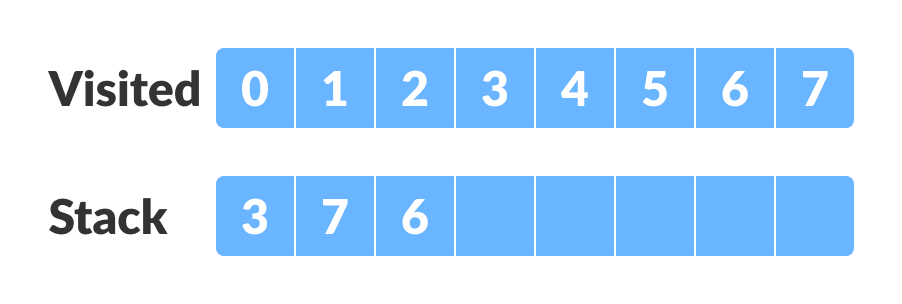
Stacking
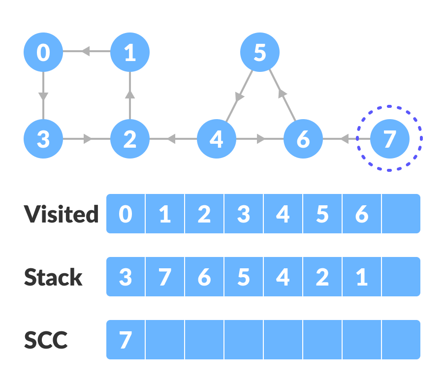
Similarly, a final stack is created.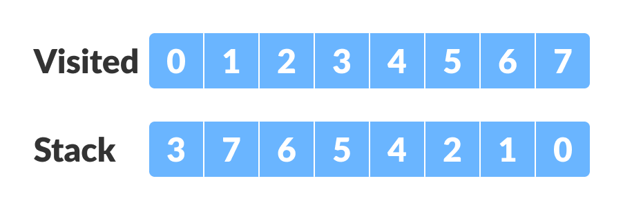
Final Stack - Reverse the original graph.
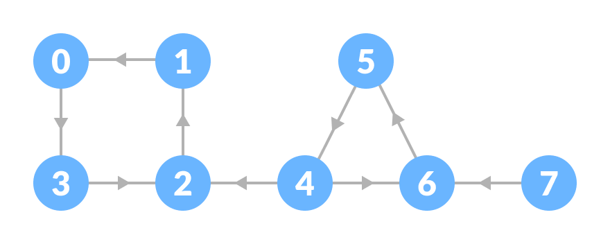
DFS on reversed graph - Perform depth-first search on the reversed graph.
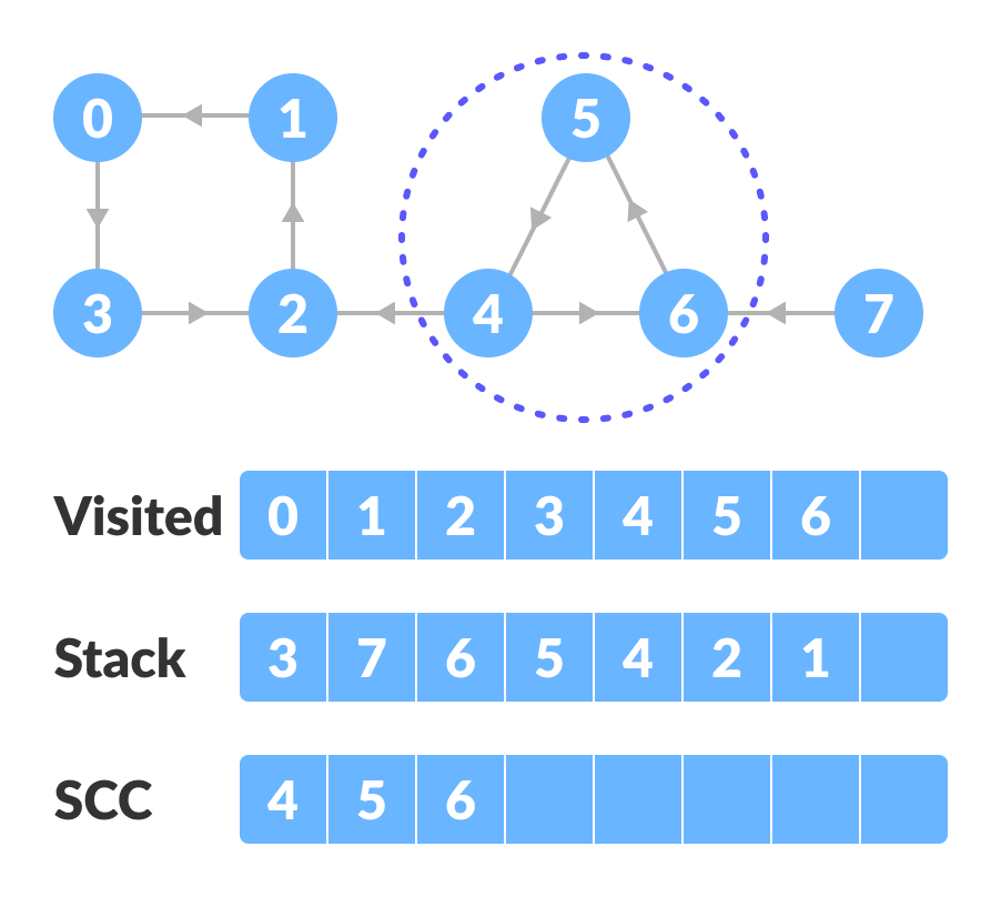
Start from the top vertex of the stack. Traverse through all of its child vertices. Once the already visited vertex is reached, one strongly connected component is formed.
For example: Pop vertex-0 from the stack. Starting from vertex-0, traverse through its child vertices (vertex-0, vertex-1, vertex-2, vertex-3 in sequence) and mark them as visited. The child of vertex-3 is already visited, so these visited vertices form one strongly connected component.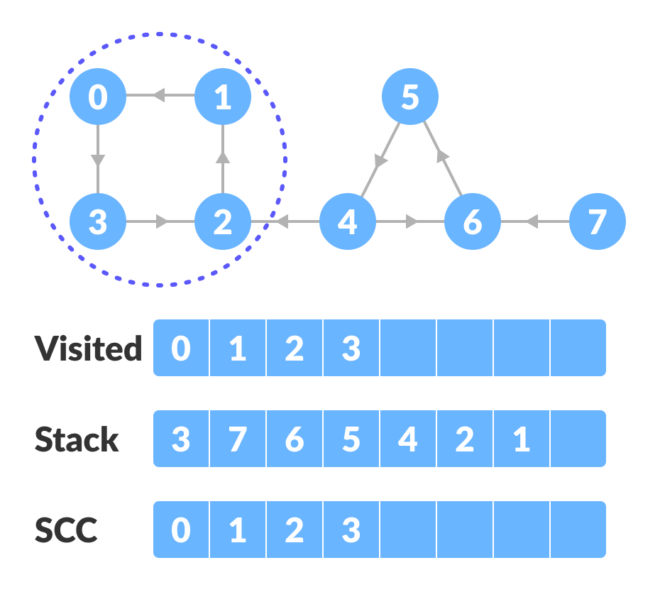
Start from the top and traverse through all the vertices
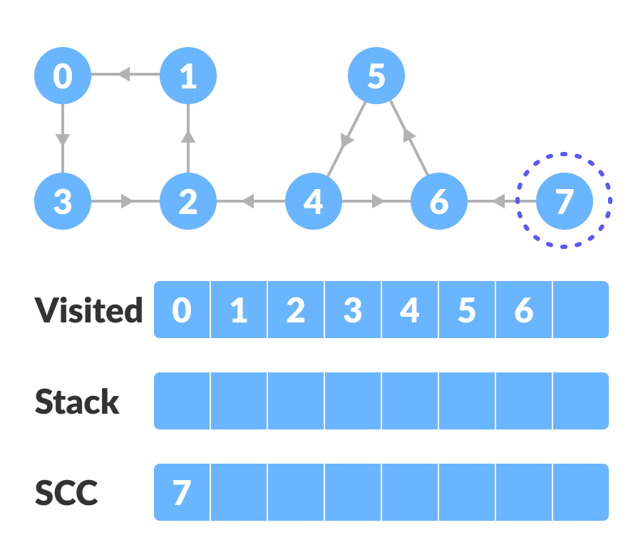
Go to the stack and pop the top vertex if already visited. Otherwise, choose the top vertex from the stack and traverse through its child vertices as presented above.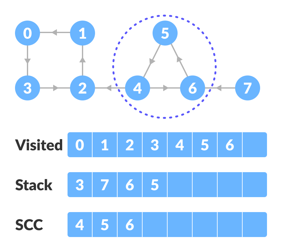
Pop the top vertex if already visited 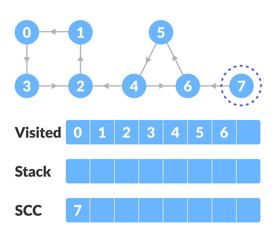
Strongly connected component - Thus, the strongly connected components are:
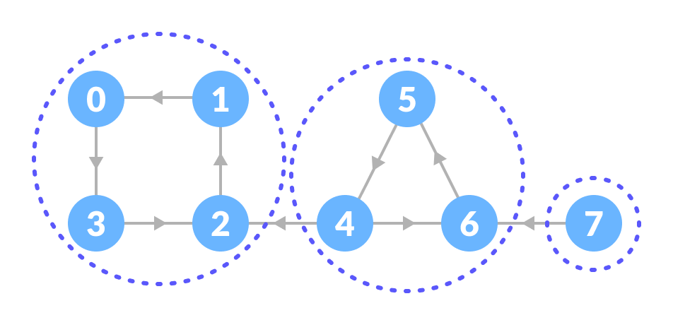
All strongly connected components
Python, Java, C++ examples
# Kosaraju's algorithm to find strongly connected components in Python


from collections import defaultdict

class Graph:

    def __init__(self, vertex):
        self.V = vertex
        self.graph = defaultdict(list)

    # Add edge into the graph
    def add_edge(self, s, d):
        self.graph[s].append(d)

    # dfs
    def dfs(self, d, visited_vertex):
        visited_vertex[d] = True
        print(d, end='')
        for i in self.graph[d]:
            if not visited_vertex[i]:
                self.dfs(i, visited_vertex)

    def fill_order(self, d, visited_vertex, stack):
        visited_vertex[d] = True
        for i in self.graph[d]:
            if not visited_vertex[i]:
                self.fill_order(i, visited_vertex, stack)
        stack = stack.append(d)

    # transpose the matrix
    def transpose(self):
        g = Graph(self.V)

        for i in self.graph:
            for j in self.graph[i]:
                g.add_edge(j, i)
        return g

    # Print stongly connected components
    def print_scc(self):
        stack = []
        visited_vertex = [False] * (self.V)

        for i in range(self.V):
            if not visited_vertex[i]:
                self.fill_order(i, visited_vertex, stack)

        gr = self.transpose()

        visited_vertex = [False] * (self.V)

        while stack:
            i = stack.pop()
            if not visited_vertex[i]:
                gr.dfs(i, visited_vertex)
                print("")


g = Graph(8)
g.add_edge(0, 1)
g.add_edge(1, 2)
g.add_edge(2, 3)
g.add_edge(2, 4)
g.add_edge(3, 0)
g.add_edge(4, 5)
g.add_edge(5, 6)
g.add_edge(6, 4)
g.add_edge(6, 7)

print("Strongly Connected Components:")
g.print_scc()
// Kosaraju's algorithm to find strongly connected components in Java

import java.util.*;
import java.util.LinkedList;

class Graph {
	private int V;
	private LinkedList<Integer> adj[];

	// Create a graph
	Graph(int s) {
		V = s;
		adj = new LinkedList[s];
		for (int i = 0; i < s; ++i)
			adj[i] = new LinkedList();
	}

  // Add edge
	void addEdge(int s, int d) {
		adj[s].add(d);
	}

	// DFS
	void DFSUtil(int s, boolean visitedVertices[]) {
		visitedVertices[s] = true;
		System.out.print(s + " ");
		int n;

		Iterator<Integer> i = adj[s].iterator();
		while (i.hasNext()) {
			n = i.next();
			if (!visitedVertices[n])
				DFSUtil(n, visitedVertices);
		}
	}

	// Transpose the graph
	Graph Transpose() {
		Graph g = new Graph(V);
		for (int s = 0; s < V; s++) {
			Iterator<Integer> i = adj[s].listIterator();
			while (i.hasNext())
				g.adj[i.next()].add(s);
		}
		return g;
	}

	void fillOrder(int s, boolean visitedVertices[], Stack stack) {
		visitedVertices[s] = true;

		Iterator<Integer> i = adj[s].iterator();
		while (i.hasNext()) {
			int n = i.next();
			if (!visitedVertices[n])
				fillOrder(n, visitedVertices, stack);
		}
		stack.push(new Integer(s));
	}

	// Print strongly connected component
	void printSCC() {
		Stack stack = new Stack();

		boolean visitedVertices[] = new boolean[V];
		for (int i = 0; i < V; i++)
			visitedVertices[i] = false;

		for (int i = 0; i < V; i++)
			if (visitedVertices[i] == false)
				fillOrder(i, visitedVertices, stack);

		Graph gr = Transpose();

		for (int i = 0; i < V; i++)
			visitedVertices[i] = false;

		while (stack.empty() == false) {
			int s = (int) stack.pop();

			if (visitedVertices[s] == false) {
				gr.DFSUtil(s, visitedVertices);
				System.out.println();
			}
		}
	}

	public static void main(String args[]) {
		Graph g = new Graph(8);
		g.addEdge(0, 1);
		g.addEdge(1, 2);
		g.addEdge(2, 3);
		g.addEdge(2, 4);
		g.addEdge(3, 0);
		g.addEdge(4, 5);
		g.addEdge(5, 6);
		g.addEdge(6, 4);
		g.addEdge(6, 7);

		System.out.println("Strongly Connected Components:");
		g.printSCC();
	}
}
// Kosaraju's algorithm to find strongly connected components in C++

#include <iostream>
#include <list>
#include <stack>

using namespace std;

class Graph {
  int V;
  list<int> *adj;
  void fillOrder(int s, bool visitedV[], stack<int> &Stack);
  void DFS(int s, bool visitedV[]);

   public:
  Graph(int V);
  void addEdge(int s, int d);
  void printSCC();
  Graph transpose();
};

Graph::Graph(int V) {
  this->V = V;
  adj = new list<int>[V];
}

// DFS
void Graph::DFS(int s, bool visitedV[]) {
  visitedV[s] = true;
  cout << s << " ";

  list<int>::iterator i;
  for (i = adj[s].begin(); i != adj[s].end(); ++i)
    if (!visitedV[*i])
      DFS(*i, visitedV);
}

// Transpose
Graph Graph::transpose() {
  Graph g(V);
  for (int s = 0; s < V; s++) {
    list<int>::iterator i;
    for (i = adj[s].begin(); i != adj[s].end(); ++i) {
      g.adj[*i].push_back(s);
    }
  }
  return g;
}

// Add edge into the graph
void Graph::addEdge(int s, int d) {
  adj[s].push_back(d);
}

void Graph::fillOrder(int s, bool visitedV[], stack<int> &Stack) {
  visitedV[s] = true;

  list<int>::iterator i;
  for (i = adj[s].begin(); i != adj[s].end(); ++i)
    if (!visitedV[*i])
      fillOrder(*i, visitedV, Stack);

  Stack.push(s);
}

// Print strongly connected component
void Graph::printSCC() {
  stack<int> Stack;

  bool *visitedV = new bool[V];
  for (int i = 0; i < V; i++)
    visitedV[i] = false;

  for (int i = 0; i < V; i++)
    if (visitedV[i] == false)
      fillOrder(i, visitedV, Stack);

  Graph gr = transpose();

  for (int i = 0; i < V; i++)
    visitedV[i] = false;

  while (Stack.empty() == false) {
    int s = Stack.top();
    Stack.pop();

    if (visitedV[s] == false) {
      gr.DFS(s, visitedV);
      cout << endl;
    }
  }
}

int main() {
  Graph g(8);
  g.addEdge(0, 1);
  g.addEdge(1, 2);
  g.addEdge(2, 3);
  g.addEdge(2, 4);
  g.addEdge(3, 0);
  g.addEdge(4, 5);
  g.addEdge(5, 6);
  g.addEdge(6, 4);
  g.addEdge(6, 7);

  cout << "Strongly Connected Components:\n";
  g.printSCC();
}
Kosaraju's Algorithm Complexity
Kosaraju's algorithm runs in linear time i.e. O(V+E).
Strongly Connected Components Applications
- Vehicle routing applications
- Maps
- Model-checking in formal verification
Divide and Conquer Algorithm
A divide and conquer algorithm is a strategy of solving a large problem by
- breaking the problem into smaller sub-problems
- solving the sub-problems, and
- combining them to get the desired output.
To use the divide and conquer algorithm, recursion is used. Learn about recursion in different programming languages:
Do you want to learn Recursion the right way? Enroll in our Interactive Recursion Course for FREE.
How Divide and Conquer Algorithms Work?
Here are the steps involved:
- Divide: Divide the given problem into sub-problems using recursion.
- Conquer: Solve the smaller sub-problems recursively. If the subproblem is small enough, then solve it directly.
- Combine: Combine the solutions of the sub-problems that are part of the recursive process to solve the actual problem.
Let us understand this concept with the help of an example.
Here, we will sort an array using the divide and conquer approach (ie. merge sort).
- Let the given array be:
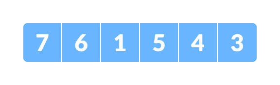
Array for merge sort - Divide the array into two halves.
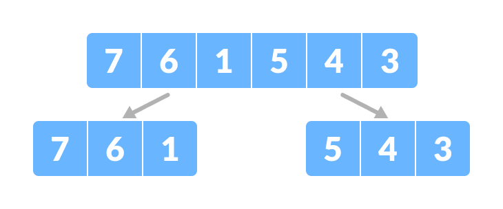
Divide the array into two subparts
Again, divide each subpart recursively into two halves until you get individual elements.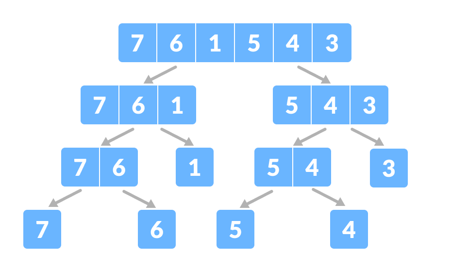
Divide the array into smaller subparts - Now, combine the individual elements in a sorted manner. Here, conquer and combine steps go side by side.
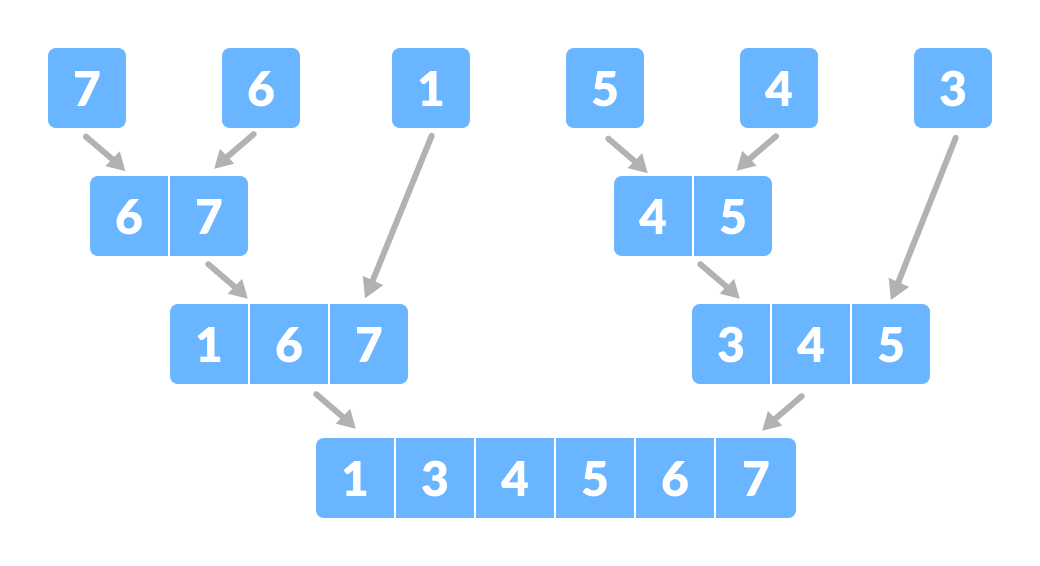
Combine the subparts
Time Complexity
The complexity of the divide and conquer algorithm is calculated using the master theorem.
T(n) = aT(n/b) + f(n),
where,
n = size of input
a = number of subproblems in the recursion
n/b = size of each subproblem. All subproblems are assumed to have the same size.
f(n) = cost of the work done outside the recursive call, which includes the cost of dividing the problem and cost of merging the solutions
Let us take an example to find the time complexity of a recursive problem.
For a merge sort, the equation can be written as:
T(n) = aT(n/b) + f(n)
     = 2T(n/2) + O(n)
Where,
a = 2 (each time, a problem is divided into 2 subproblems)
n/b = n/2 (size of each sub problem is half of the input)
f(n) = time taken to divide the problem and merging the subproblems
T(n/2) = O(n log n) (To understand this, please refer to the master theorem.)

Now, T(n) = 2T(n log n) + O(n)
          ≈ O(n log n)
Divide and Conquer Vs Dynamic approach
The divide and conquer approach divides a problem into smaller subproblems; these subproblems are further solved recursively. The result of each subproblem is not stored for future reference, whereas, in a dynamic approach, the result of each subproblem is stored for future reference.
Use the divide and conquer approach when the same subproblem is not solved multiple times. Use the dynamic approach when the result of a subproblem is to be used multiple times in the future.
Let us understand this with an example. Suppose we are trying to find the Fibonacci series. Then,
Divide and Conquer approach:
fib(n)
    If n < 2, return 1
    Else , return f(n - 1) + f(n -2)
Dynamic approach:
mem = []
fib(n)
    If n in mem: return mem[n]
    else,
        If n < 2, f = 1
        else , f = f(n - 1) + f(n -2)
        mem[n] = f
        return f
In a dynamic approach, mem stores the result of each subproblem.
Advantages of Divide and Conquer Algorithm
- The complexity for the multiplication of two matrices using the naive method is O(n3), whereas using the divide and conquer approach (i.e. Strassen's matrix multiplication) is O(n2.8074). This approach also simplifies other problems, such as the Tower of Hanoi.
- This approach is suitable for multiprocessing systems.
- It makes efficient use of memory caches.
Divide and Conquer Applications
- Binary Search
- Merge Sort
- Quick Sort
- Strassen's Matrix multiplication
- Karatsuba Algorithm
Do you want to learn Recursion the right way? Enroll in our Interactive Recursion Course for FREE.
Master Theorem
The master method is a formula for solving recurrence relations of the form:
T(n) = aT(n/b) + f(n),
where,
n = size of input
a = number of subproblems in the recursion
n/b = size of each subproblem. All subproblems are assumed
     to have the same size.
f(n) = cost of the work done outside the recursive call,
      which includes the cost of dividing the problem and
      cost of merging the solutions

Here, a ≥ 1 and b > 1 are constants, and f(n) is an asymptotically positive function.
An asymptotically positive function means that for a sufficiently large value of n, we have f(n) > 0.
The master theorem is used in calculating the time complexity of recurrence relations (divide and conquer algorithms) in a simple and quick way.
Master Theorem
If a ≥ 1 and b > 1 are constants and f(n) is an asymptotically positive function, then the time complexity of a recursive relation is given by
T(n) = aT(n/b) + f(n)

where, T(n) has the following asymptotic bounds:

    1. If f(n) = O(nlogb a-ϵ), then T(n) = Θ(nlogb a).

    2. If f(n) = Θ(nlogb a), then T(n) = Θ(nlogb a * log n).

    3. If f(n) = Ω(nlogb a+ϵ), then T(n) = Θ(f(n)).

ϵ > 0 is a constant.
Each of the above conditions can be interpreted as:
- If the cost of solving the sub-problems at each level increases by a certain factor, the value of
f(n)will become polynomially smaller thannlogb a. Thus, the time complexity is oppressed by the cost of the last level ie.nlogb a - If the cost of solving the sub-problem at each level is nearly equal, then the value of
f(n)will benlogb a. Thus, the time complexity will bef(n)times the total number of levels ie.nlogb a * log n - If the cost of solving the subproblems at each level decreases by a certain factor, the value of
f(n)will become polynomially larger thannlogb a. Thus, the time complexity is oppressed by the cost off(n).
Solved Example of Master Theorem
T(n) = 3T(n/2) + n2
Here,
a = 3
n/b = n/2
f(n) = n2

logb a = log2 3 ≈ 1.58 < 2

ie. f(n) > nlogb a+ϵ , where, ϵ is a constant.

Case 3 implies here.

Thus, T(n) = f(n) = Θ(n2)
Master Theorem Limitations
The master theorem cannot be used if:
- T(n) is not monotone. eg.
T(n) = sin n f(n)is not a polynomial. eg.f(n) = 2n- a is not a constant. eg.
a = 2n a < 1
- Solved Example of Master Theorem
- Master Theorem
- Solved Example of Master Theorem
- Master Theorem Limitations
Asymptotic Analysis: Big-O Notation and More
The efficiency of an algorithm depends on the amount of time, storage and other resources required to execute the algorithm. The efficiency is measured with the help of asymptotic notations.
An algorithm may not have the same performance for different types of inputs. With the increase in the input size, the performance will change.
The study of change in performance of the algorithm with the change in the order of the input size is defined as asymptotic analysis.
Do you want to learn Time Complexity the right way? Enroll in our Interactive Complexity Calculation Course for FREE.
Asymptotic Notations
Asymptotic notations are the mathematical notations used to describe the running time of an algorithm when the input tends towards a particular value or a limiting value.
For example: In bubble sort, when the input array is already sorted, the time taken by the algorithm is linear i.e. the best case.
But, when the input array is in reverse condition, the algorithm takes the maximum time (quadratic) to sort the elements i.e. the worst case.
When the input array is neither sorted nor in reverse order, then it takes average time. These durations are denoted using asymptotic notations.
There are mainly three asymptotic notations:
- Big-O notation
- Omega notation
- Theta notation
Big-O Notation (O-notation)
Big-O notation represents the upper bound of the running time of an algorithm. Thus, it gives the worst-case complexity of an algorithm.
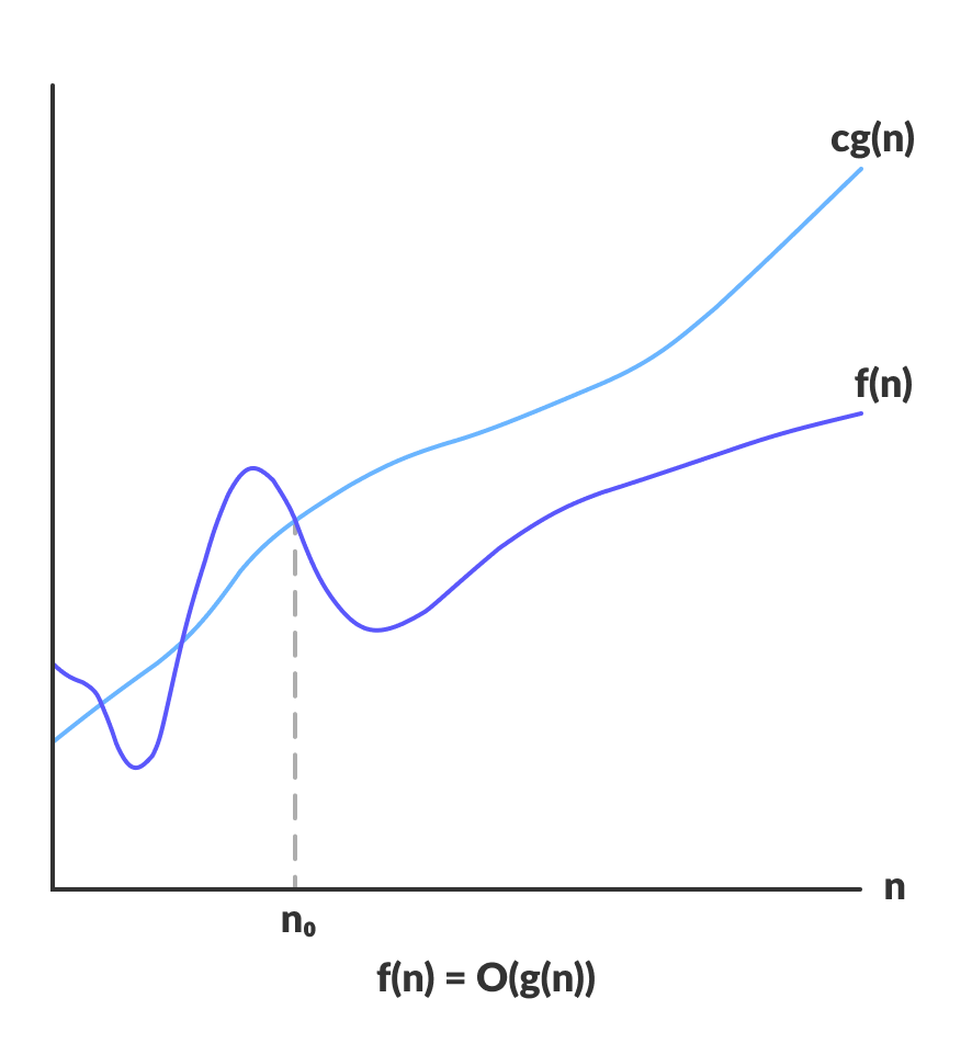
O(g(n)) = { f(n): there exist positive constants c and n0
            such that 0 ≤ f(n) ≤ cg(n) for all n ≥ n0 }
The above expression can be described as a function f(n) belongs to the set O(g(n)) if there exists a positive constant c such that it lies between 0 and cg(n), for sufficiently large n.
For any value of n, the running time of an algorithm does not cross the time provided by O(g(n)).
Since it gives the worst-case running time of an algorithm, it is widely used to analyze an algorithm as we are always interested in the worst-case scenario.
Omega Notation (Ω-notation)
Omega notation represents the lower bound of the running time of an algorithm. Thus, it provides the best case complexity of an algorithm.
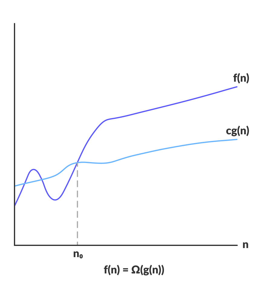
Ω(g(n)) = { f(n): there exist positive constants c and n0
            such that 0 ≤ cg(n) ≤ f(n) for all n ≥ n0 }
The above expression can be described as a function f(n) belongs to the set Ω(g(n)) if there exists a positive constant c such that it lies above cg(n), for sufficiently large n.
For any value of n, the minimum time required by the algorithm is given by Omega Ω(g(n)).
Theta Notation (Θ-notation)
Theta notation encloses the function from above and below. Since it represents the upper and the lower bound of the running time of an algorithm, it is used for analyzing the average-case complexity of an algorithm.
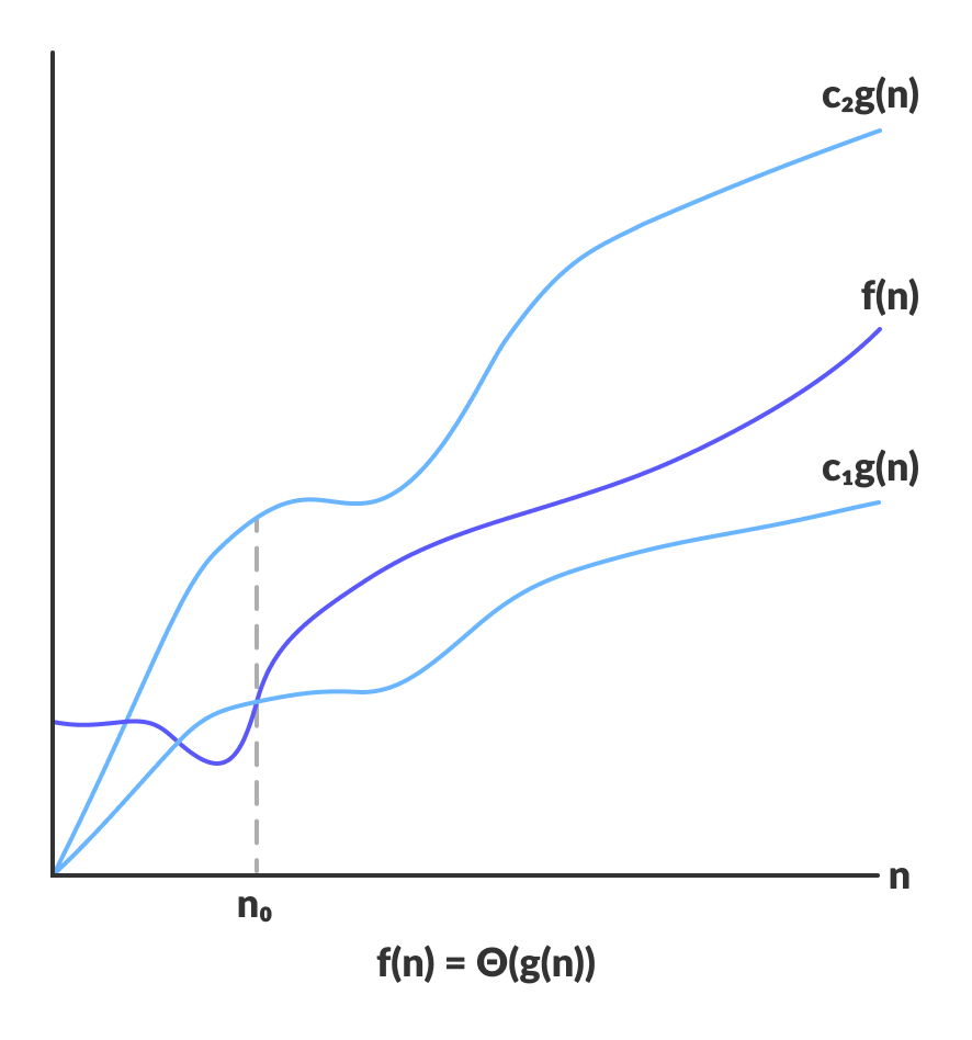
For a function g(n), Θ(g(n)) is given by the relation:
Θ(g(n)) = { f(n): there exist positive constants c1, c2 and n0
            such that 0 ≤ c1g(n) ≤ f(n) ≤ c2g(n) for all n ≥ n0 }
The above expression can be described as a function f(n) belongs to the set Θ(g(n)) if there exist positive constants c1 and c2 such that it can be sandwiched between c1g(n) and c2g(n), for sufficiently large n.
If a function f(n) lies anywhere in between c1g(n) and c2g(n) for all n ≥ n0, then f(n) is said to be asymptotically tight bound.
Do you want to learn Time Complexity the right way? Enroll in our Interactive Complexity Calculation Course for FREE.